PREFACE

From dehydrating floodplain nature to climate proof water supply

When reviewing the articles, the editorial board consisting of experts from the sector made a selection, looking for a clear relationship with daily practice in the water sector, which is the purpose of Water Matters. Research, results and findings form the basis for articles that describe new knowledge, insights and technologies with a view to practical use.
This edition once again covers a wide range of topics. From the dehydration of floodplain nature ('uniformity threatens') and the threat to the iconic fire salamander by a deadly fungus to the experiences with the sludge digestion technology Ephyra, and the load of slaughterhouse wastewater on the Nereda installation at rwzi Epe.
But also: a method to get a grip on the growing toxic pressure on water, a forecasting tool for the replacement of wet civil engineering works, insight into phosphate concentrations in groundwater under agricultural land (the standards are rarely exceeded), climate proof water supply with decentralised water supply, a comparison test of nitrate sensors, a monitoring module for fish migration and a new predictive lab method for dewatering at wastewater treatment plants.
Water Matters is, just like the professional journal H₂O, an initiative of the Royal Dutch Water Network (KNW), the independent knowledge network for and by Dutch water professionals. Members of KNW receive Water Matters twice a year as a free supplement to their magazine H₂O.
The publication of Water Matters is made possible by leading players in the Dutch water sector. These Founding Partners are ARCADIS, Deltares, KWR Water Research Institute, Royal HaskoningDHV and Stichting Toegepast Onderzoek Waterbeheer (STOWA). With the publication of Water Matters the participating institutions want to make new, applicable water knowledge accessible.

You can also read Water Matters digitally on H2O-online (www.h2owaternetwerk.nl). In addition, this publication is also available in English as a digital magazine via the same website or via www.h2o-watermatters.com.
The English articles can be shared from the digital magazine on H₂O-online. Furthermore, articles from previous editions can be found on the site.

Enjoy reading this edition. Would you like to respond? Please let us know via redactie@h2o-media.nl.

Monique Bekkenutte Publisher (Royal Dutch Water Network)
Huib de Vriend Chairman editorial board Water Matters

Reduced variety of floodplain nature: a threat of uniformity!

The Netherlands increasingly have to deal with larger variations in river discharges due to climate change. At the same time, the river bed is eroding and the floodplains are silting up as a result of historic human interventions. These developments contribute to the desiccation of floodplains and consequently threaten the characteristic Dutch riverine nature. This article describes the impact of these developments on the condition of Dutch terrestrial floodplain nature and the potential design and management measures that could be taken to counteract the negative effects.

Various developments are imposing pressures on our river system. Climate change causes river discharges to become both higher and (prolonged) lower. Embankments and normalisations in recent centuries have resulted in the river to be narrower and this reduced the extent of the floodplains. This process reduced discharge capacities significantly. Another effect is that a much narrower river relates to more gentle river bed slopes to which the river gradually adapts. Due to embankments on both sides of the river, the river can only adapt by eroding the river bed and by releasing sediments on the floodplain during high water. This is a self-reinforcing process with ever-increasing consequences for water safety, fresh water supply, shipping, nature and many other functions that depend on (ground) water levels.

River bed erosion results in lower water levels on sections without weirs, lower ground water levels in floodplains, less frequent inundation of floodplains and a reduction of dynamics that are vital for nature. Floodplains desiccate as a consequence and this causes a loss in diversity of floodplain nature. This river bed erosion in combination with climate change, which is related to lower water levels during summer and higher water levels in spring and fall, can have significant consequences for the valuable riverine nature in The Netherlands.

This exploratory study shows which groundwater conditions are needed for the different types of nature in floodplains, what the current and future conditions are, and with which design and management measures these conditions can be realised. For the assessment of floodplain nature this study used ecotopes: relatively homogeneous, spatial vegetation types that have roughly the same environmental demands.

Methods

Based on literature study and a session with ecologists and vegetation experts, ground water conditions required for the ecological functioning of terrestrial floodplain nature were identified. Subsequently, the conditions were compared with the current and future hydrological conditions in the floodplains. These were simulated with the National Water Model, which also includes a ground water model. Climate effects were investigated using the future scenarios of the Deltaprogramma Zoetwater (English: Delta Program Freshwater). The extent of river bed erosion was based on annual bed measurements and extrapolated for future scenarios. This shows an erosional trend of approximately one to two centimetres per year (the extent differs greatly along the river; both per river branch and per river).

An ecotope map (5th edition) was used to map floodplain nature. The following five terrestrial ecotope types, relevant for the study area, were distinguished: hardwood forests and shrubs, softwood forests and shrubs, wet grasslands, dry grasslands, and reeds and marshes. These ecotope types can roughly be categorised as wet (wet grasslands and reeds/marshes) and dry nature (dry grasslands and hardwood forests/shrubs), with softwood forests and shrubs in an intermediate position. The (future) suitability of the locations for the ecotope types was assessed using the calculated average spring ground water levels (GVG) in the current situation and the year 2050 (based on the Steam scenario of the Deltaprogramma Zoetwater). The GVG was chosen because of the importance of the spring ground water level for the development of vegetation and its reliability as a boundary condition for each ecotope type. Two scenarios have been taken into account for 2050: a situation without river bed management (in other words: ongoing erosion) and a situation with management in which the river bed is kept on its current level. The assessments are categorised as: too wet, wet, good, dry and too dry.

Gelderse Poort

The Programmatische Aanpak Grote Wateren (PAGW, English: Programmatic Approach Large Waters) has investigated what is needed to realise a robust and futureproof river system. The outcome of this program is part of the program Integraal Rivier Management (IRM, English: Integral River Management). The PAGW study resulted in four hotspots (Biesbosch, IJssel-Vechtdelta, Grensmaas and Gelderse Poort) that form the base for ecological improvement of the river area (Van der Sluis et al., 2020). The methods for the assessment of hydrological conditions of ecotopes was applied to the Gelderse Poort as river bed erosion is most evident in this area: the eroding stretches of the Waalbochten, the Pannerdens Kanaal and the Boven-Ijssel are adjacent to the Gelderse Poort. The area of the Gelderse Poort further includes the Oude Rijn and Groenlanden because of the closely related ecology and the potential to achieve sustainable populations of species in low-dynamic ecotopes.

Current condition of floodplain nature

In the past centuries, the river bed in the Gelderse Poort has eroded with one to two metres. For ecotopes that prefer wet conditions, this erosion has already led to a severe degradation (Fig. 1, current situation). For the ecotope reeds and marshes the spring ground water levels are too low and the situation is too dry. The hydrological conditions are more suitable for the dry ecotope types and in some locations even (too) wet. Softwood forests and shrubs thrive in a wide range of hydrological conditions: for this ecotope type the conditions on the present locations are on the dry side, but still acceptable. This analysis is based on an assessment of the average spring ground water levels only and does not consider other aspects in relation to the location of ecotopes, such as soil type, inundation frequency and the level of continuity. These aspects also determine whether or not a location is suitable for an ecotope (e.g. hardwood forests and shrubs require a higher location with a low flood frequency of less than once every 10 years). Our conclusions thus only focus on the ground water level.

Future condition of floodplain nature

The effect of climate change on spring river discharge is relatively small in the climate scenarios considered (Fig. 2). This means that the effect of climate change on mean spring ground water levels is also limited. As a result, there are hardly any differences between the assessment of the hydrological conditions in the current situation and the future situation in 2050 (with only the climate effect, right column in Fig. 1). Due to the ongoing river bed erosion, conditions become drier in floodplain. This desiccation causes the conditions for dry ecotopes to improve, while the conditions for wet ecotopes deteriorate (fig. 1). This threatens the characteristic wet river nature and will lead to a decrease in the variety of floodplain nature: homogeneity is therefore imminent.

Perspective

Two types of measures are possible to ensure that the floodplain will regain its needed wet conditions. The first one is to bring the river water level and the floodplain level closer together. Maintaining the present level of the river bed is crucial and should be combined with raising the bed level where possible. Additionally, the floodplain level can be lowered when redesigning floodplains. This way additional relief and variation can be regained in the floodplain such that the higher and dryer habitats remain suitable for the dry ecotopes. The second type of measures focuses on retaining water for a longer period of time in the floodplain in spring and early summer. By managing inlets differently, water can be let in and out in a controlled manner, which could lengthen the inundation period and keeping the ground water levels higher. This is beneficial for the low-dynamic reeds and marshes situated in these areas. Both types of measures will increase hydrodynamics. It will be necessary to combine several interventions to achieve an optimal ecotope distribution.

Conclusions

In the present situation, wetland ecotopes have already dried out considerably and may disappear from the Dutch river landscape in the future. Climate change in combination with river bed erosion increases the desiccation of floodplains which threatens the characteristic wet river nature. This may lead to a decrease in the variety of floodplain nature: homogeneity is imminent. The concern of Rijkswaterstaat is that targets set up for nature (described in the Natura 2000 management plans and executed in the PAGW) will be under pressure.
This exploratory study shows that it is of great importance to stop river bed erosion. This can be done by active river bed management. Other measures to limit desiccation of floodplains are lowering the floodplain level or retaining water for a longer period of time. It is crucial to elaborate these measures. The method described in this article can be used to assess the effectiveness of the measures and also perform an assessment for other PAGW hotspots and floodplain areas along the Rhine and the Meuse.

Kris van den Berg
(Rijkswaterstaat)
Marieke de Lange
(Rijkswaterstaat)
Saskia van Vuren
(Rijkswaterstaat)

Summary

River bed erosion has already led to deterioration of characteristic floodplain nature. Without intervention, this ongoing erosion in combination with lower discharges in summer due to climate change, will lead to further deterioration, especially of wet ecotope types. Managing the river bed at the present bed level will limit further damage. Other types of design and management measures are needed to improve the hydrological conditions in floodplains and make floodplains suitable again for both wet and dry ecotopes.

References

Klijn, F., Hegnauer, M., Beersma, J., & Sperna Weiland, F. (2015). What do new climate scenarios mean to the river discharges of the Rhine and Meuse? A summary of the GRADE research on implications of new climate projections for river discharges. Deltares & KNMI, Delft. Report nr. 1220042-004. Wat betekenen de nieuwe klimaatscenario's voor de rivierafvoeren van Rijn en Maas? (deltares.nl)

Van den Berg, K. (2021). Hydrological and hydraulic boundary conditions for nature development in floodplains. Method development and application on the Gelderse Poort. Rijkswaterstaat, Lelystad. Hydrologische en hydraulische randvoorwaarden voor natuurontwikkeling en -behoud in uiterwaarden : methodiek ontwikkeling en toepassing op Gelderse Poort - Rijkswaterstaat Rapportendatabank (overheid.nl)

Van der Sluis, T., Pedroli, B., Woltjer, I., Van Elburg, E. & Maas, G. (2020). Elaboration on the PAGW Nature Analysis Hotspots Large Rivers; Final Report. Wageningen: Wageningen Environmental Research, report 3031. https://edepot.wur.nl/534790

Wolters, H. A., Van Der Born, G. J., Dammers, E., Reinhard, S. (2018). Delta scenarios for the 21st century, actualisation 2017. Deltares, Utrecht. Deltascenarios_actualisering2017_hoofdrapport.pdf (deltares.nl)

^ Back to start

The result of 10 years experience with Ephyra sludge digestion

A new sludge digester has been in operation at the Tollebeek waste water treatment plant in Flevoland since 2017. The digester is an Ephyra system, developed since 2010 by Royal HaskoningDHV. Instead of one mixed reactor, the system use 3 or 4 reactors in series, resulting in a more complete digestion and a higher biogas production.

This new sludge digestion method was developed as a part of ‘the Energy factory’ concept, an energy-neutral or even energy-producing sewage treatment plant. During the technology development, special attention was given to:
• performance under different conditions, including different types of sludge and varying sludge retention times;
• sludge digestion and biogas production and how they compare to the performance of other sludge digestion technologies;
• stability at different sludge loads and retention times.
In this article, we discuss the operation and performance of Ephyra with respect of the aforementioned questions, and particular focus on the development from lab to full scale.

Figure 1. Principle of the Ephyra technology, with 3 reactors as compartments in one digestion tank. A serial configuration of separate tanks is also possible.

Operation

The principle of Ephyra sludge digestion is based on operating 2 to 4 reactors or compartments in series, rather than a single mixed reactor or tank (see Figure 1). This way a plug flow type of digestion is created. When compared to a single completely mixed tank, a plug flow digestion gives fewer short-circuiting, sludge degradation proceeds more quickly, and the individual phases of the sludge digestion process are more separated and optimised in the different reactors. This all leads to a better digestion with more sludge breakdown and more biogas.
Another important advantage of Ephyra is that average retention times of 6 to 7 days are feasible, instead of the usual 15 to 20 days. As a result, the capacity of the system is high and more sludge can be processed with the same reactor volume. The shorter retention times are possible using a process control including a recirculation from the last to the first reactor of the series ; this control strategy helps to prevent problems including acidification in the first reactor.

From lab to full scale

The development of Ephyra started around 2010, with the first ideas and creation of a calculation model. The results of the first technical model calculations confirmed the expected benefits over a completely mixed reactor, namely better sludge digestion and more biogas production. To validate the model results, various tests with batch and continuous systems were done at Royal HaskoningDHV's Technological Research Centre. A number of different sludge types were tested, with different ratios of primary sludge (from pre-sedimentation) and secondary sludge (from an activated sludge system). Comparison with conventional mesophilic digestion once again demonstrated that sludge breakdown was much higher. In Ephyra systems, when only secondary sludge was digested, 15% more sludge was broken down, with 15% higher biogas production at the same time

2014-2016: pilot project at Tollebeek waste water treatment plant

The results of the technical and financial model calculations and the lab tests were for Royal HaskoningDHV and the Zuiderzeeland Water authority reason to conduct a pilot study at the Tollebeek waste water treatment plant. The idea was that, if the pilot test was to prove successful, Ephyra sludge digestion could be applied at this waste water treatment plant and that sludge from Lelystad could also be digested here in the future. This would be possible by expanding the existing digestion at Tollebeek with an Ephyra digestion tank before the existing one.
The pilot system consisted of four mechanically mixed reactors connected in series, with an internal controlled recirculation from the last to the first reactor. The total retention time was around 7 to 8 days; the retention time per reactor around 2 days. The pilot showed that the sludge breakdown, averaging 40% dry solids, was in line with expectations.
During the pilot test peak loadings were also tested, with the total retention time reduced to 5 days for periods of 5 to 10 days. During these periods of peak loading, the system continued to function stable; there was no noticeable drop in pH and sludge breakdown and biogas production remained steady; process control of the internal recirculation system functioned properly (see Stowa report 2016-34).
In addition to the pilot project, we also carried out model calculations involving various configurations and arrangements for use of the Ephyra digester at the Tollebeek waste water treatment plant; examples are the number of reactors in series and the degree of internal recirculation.

From pilot to design

The results of the pilot test and the model calculations were used to make a final design for the full scale system for Tollebeek. This design differed from the orginal 2010 draft.

Use of horizontal mixed reactors
The original design was based on vertical reactors compartmentalised by partitions. However, this proved to have a number of drawbacks. The accessibility of the reactors (compartments) for maintenance was difficult, the reactors were higher than the building heights for sludge digesters used in the Netherlands, and the partitions were sensitive to blockages. The system was also expensive. A design with horizontal reactors connected in series did not have any of these drawbacks. This decision had already been taken prior to the pilot and the pilot system had been adapted to take these changes into account.

3 instead of 4 reactors in series
The model calculations indicated that there was almost no difference between the performance of 3 rather than 4 reactors in series. This was confirmed by lab tests. In view of the simplicity of the system and with cost considerations in mind, it was decided that 3 reactors in series (in a single tank) was the most appropriate for Tollebeek. Using 3 reactors in series has since then become the standard when constructing a completely new Ephyra sludge digester. If retrofitting existing systems, a different design is possible. The 3 reactors / compartments in the full scale system at Tollebeek have been constructed as slices of a pie, hydraulically connected in 1 reactor with a total volume of 1,500 m3.

Thickened sludge properties and design
In addition to the aforementioned design aspects, the pilot study also indicated that sludge, and thicker sludge in particular (as used in sludge digestion), is a ‘special’ medium with a relatively high viscosity. This is important for the design of mixers, pumps, heat exchangers and other equipment, piping and valves.

The Ephyra full scale plant at Tollebeek was completed at the end of 2017 and is functioning well. A second full scale plant has been operational since 2021 as an integral part of the Energy Plant at the Sleeuwijk waste water treatment plant. This is a completely new system (‘green field situation’) and also features 3 reactors connected in series in a single tank. In addition, two international digesters are in the design and tendering phase, and a new pilot has been started in Canada.

Figure 2. Organic matter removal (ODS) as a function of the proportion of excess sludge as measured on laboratory, pilot and full scale. 100% means that only secondary sludge is digested. The tests were carried out at approximately 15 days or more of retention time.

Figure 3. Organic matter (ODS) removal as a function of the retention time for a sludge mixture of 50% primary and 50% secondary sludge. The graph is based on laboratory tests and model calculations.

How does the Ephyra sludge digester perform?

An important parameter to evaluate sludge digestion performance is the sludge breakdown, often represented as the amount of organic dry solids (ODS) removed during the sludge digestion. This amount depends on the technology used and the sludge input type – the latter because primary sludge breaks down more effectively than secondary sludge.
The relationship between ODS removal and the percentage of secondary activated sludge in the sludge to be digested is shown in Figure 2. From this, it can be seen that if only secondary sludge is digested, approximately 45 to 46% of the organic matter is broken down. As the proportion of primary sludge increases, so too does the ODS removal. For a sludge mixture of 50% primary and 50% secondary sludge, the ODS removal is approximately 52 to 54%.
An important feature of Ephyra digesters is that they can operate and digest sludge at shorter retention times. This applies to a retention time as low as around 5 days during peak loadings. Removal efficiency is however less when using shorter retention times. The relationship between retention time and the ODS removal is shown in Figure 3. With retention times in excess of 15 days, efficiency only increases very little. The optimum lies between 10 and 15 days and depends on the composition of the sludge.
In short: the developed new way of digesting sludge with Ephyra proved to be extremely stable and reliable throughout the entire development period – on laboratory scale, during the pilot project and now in practice on full scale.

André Visser
(Royal HaskoningDHV)
Eddie Koornneef
(Royal HaskoningDHV)
Danny Traksel
(Royal HaskoningDHV)

Summary

In 2010, Royal HaskoningDHV began developing a new process for sludge digestion using the Ephyra principle. Digestion does not occur in just one completely mixed reactor but in 3 or 4 reactors in series. Laboratory-scale tests, model calculations and a pilot study resulted in a full scale design that was realised at Tollebeek waste water treatment plant in Flevoland in 2017. The new Ephyra sludge digester gives a higher breakdown of organic matter and produces more biogas than conventional digesters.

References

Stowa 2016-34. Toepassing van nieuwe gistingsconcepten Ephyra® en Themista®

^ Back to start

Invasive fungus threatens Dutch salamander with extinction

A fungal pathogen lethal to salamanders and newts has arrived from Asia in wild populations in the Netherlands. The pathogen/fungus has been known in Europe since 2013. Due to this pathogen, the fire salamander has almost disappeared from the Netherlands. Adequate detection and reporting, as well as prevention of the spread, may limit the disastrous consequences.

The fire salamander is our only terrestrial salamander. This large, iconic nocturnal animal with its black and yellow markings is (naturally) found in southern Limburg. For many years, volunteers have been monitoring the species during night-time rain showers, ideally just before or after a thunderstorm, in the Bunderbos and Vijlenerbossen forests. Beginning in 2008, the volunteers reported a striking number of dead animals and a sharp decline in the number of live animals on the transects. These observations led to the discovery of the chytrid fungus Batrachochytrium salamandrivorans (Bsal) (Martel et al., 2013; 2014). This fungus, lethal to salamanders and newts, originates in East Asia and was most likely introduced into the environment through the global trade in amphibians. What can water authorities do to prevent further spread of this fungus?

National populationtrend of the fire salamander in the Netherlands. The species has declined by 99.9% and shows no signs of recovery. Sources: RAVON, CBS

Chytridiomycosis

The Bsal fungus is not the first chytrid fungus to cause havoc outside of its natural range. Batrachochytrium dendrobatidis or Bd has caused mass mortality, particularly in Australia and South America. Both fungi cause the skin disease chytridiomycosis. This disease is considered one of the worst vertebrate infectious diseases in history, due to the combination of its high mortality rate and a broad host spectrum. Worldwide, chytridiomycosis has contributed to the decline of at least 501 species of amphibian (Scheele et al., 2019).
After infection with Bsal, the skin of a susceptible salamander is – quite literally – eaten away. Progression from infection to death in fire salamanders can occur within just two weeks, and only towards the latter stage of the disease symptoms are visible on the skin. The skin then shows black spots, often defined circles, and holes. These lesions can be very difficult to observe in darker salamanders. Furthermore, animals may also exhibit muscle spasms. The animals become lethargic but, because the process is rapid, animals can still look fine on the outside. Information sheets have been produced to help people recognise Bsal (see www.ravon.nl/bsal and www.bsaleurope.com).
The Bsal fungus is a little more robust than Bd. The latter, for example, is poorly adapted to drought, but Bsal has encysted spores that have the ability to float. This allows the fungus to survive for lengthy periods of time in water and soil, and while floating it is scarcely preyed upon by aquatic microfauna.
Brief contact of just one second is sufficient for successful Bsal transmission. Transmission can also be indirect, for instance when a Bsal-infected newt leaves the zoospores in a rain puddle, which can then infect the next salamander or newt that walks through the puddle. Humans are also effective vehicles for transmission through their boots, shoes, bicycle and car tyres. Consequently, practising good hygiene when working in the field is crucial to limit the spread of Bsal (and other pathogens). This of course applies to researchers, site managers and contractors, but also to visitors to nature reserves and participants in excursions. A final important group are the owners of garden ponds.

Early warning system

The prevalence of Bsal in ecosystems is usually low, which means that detection rate – when actively searching for an infected animal - is equally low. Since 2012, we have launched an Early Warning System (EWS) for Bsal and other herpetofauna diseases and pathogens. This EWS has proven to be an effective and cost-efficient way of detecting Bsal. The EWS operates through a hotline (see https://www.ravon.nl/Zakelijk/Ziektes). Awareness of the EWS is being raised through newsletters, local newspapers and lectures. By regularly asking as many people as possible, including site managers and water authorities, to be alert to sick and/or dead amphibians, to help recognise them and to report them, the chance of detecting an outbreak of Bsal, or any other relevant diseases, has greatly increased.
Annually, around 120 reports of sick and dead salamanders, frogs, toads and reptiles are reported via the hotline. In the event of a suspicious report, the animal can be examined and, if Bsal is found, the location and population can be actively monitored. The EWS helped to detect a new outbreak of Bsal in the province of Gelderland in 2018, some 150 kilometres from the initial outbreak site in Zuid Limburg.

The distribution of Batrachochytrium salamandrivorans in 2021. Source: RAVON

Distribution

In the Netherlands, Bsal is now known to be present in Limburg and Gelderland. Currently, the pathways of Bsal are not fully understood yet. Besides amphibian hosts that can vector the fungus, other vectors, including humans, are obvious. The distances between the current outbreak sites in the Netherlands, but also in Germany, are often quite far. This suggests that humans are currently the main spreaders, allowing the fungus to bridge large distances and barriers very quickly. Recently, Bsal has been found in fire salamanders east of the Rhine near to Essen, Germany. Within Germany, ‘jumps’ of up to 170 to 250 km have been known to occur, where natural distribution appears impossible due to the distance and other barriers.
Another possibility could be the spread via rivers, but amphibians do not inhabit the large rivers such as the Rhine and the Meuse. Moreover, the distribution of the fungus across Europe cannot be linked to rivers and, in addition, the fire salamander is a terrestrial amphibian. A recent Spanish outbreak was very clearly related to a hobbyist who had released Bsal-infected newts into the wild.

Fire salamander and crested newt

Bsal has reduced the only Dutch population of fire salamanders by 99.9%, and there’s no sign of population recovery. The fungus remains in the system (Spitzen et al., 2021). In captivity, salamanders and newts can be successfully treated by either keeping them at 25°C for a period of 10 days or by keeping them at 20°C for a period of 10 days in combination with anti-fungal treatment. Even with treatment, the animals do not develop resistance and they remain just as susceptible for a consecutive infection.
In Germany, Bsal has also reduced population sizes of the crested newt. Bsal-infected crested newt populations in the Netherlands are being monitored closely. The results of this monitoring are not yet available.

Prevention

Our current understanding is that Bsal can be cryptically present in salamander and newt populations and is not easy to detect. New introductions and further spread of Bsal must be prevented to the fullest extent possible. It is suggested that isolated fire salamander populations can be kept safe from Bsal (Spitzen van der Sluijs et al., 2018). Field-hygiene is crucial to prevent the spread of Bsal. This also means that transferring salamanders and newts (as well as other amphibians, aquatic plants and water) should be refrained from, and if it needs to be done, it should only be carried out with great restraint and care to prevent any further spread of Bsal and other pathogens (and invasive aquatic plants).
Disinfection protocols have been developed for the disinfection of large and small-scale equipment (see http://bsaleurope.com/hygiene-protocols/ and https://ravon.nl/Portals/2/Bestanden/Publicaties/Hygiene_protocol.pdf).

The future

Within the group of amphibians, 40% are threatened in their survival, making it the most endangered species group in the world today. The situation in the Netherlands is perilous. The presence of an invasive pathogen is therefore, by definition, worrying and it is vitally important that as many people as possible know that this threat exists. We can all take precautions to avoid the spread – do not move animals or aquatic plants, practise good hygiene in the field and report sick/dead salamanders, other amphibians and reptiles. Reporting allows us to carry out targeted studies. The options for preventing Bsal from entering a country or region or for mitigating the impact of an outbreak are varied (Thomas et al 2019; Martel et al 2020). At the same time, there is still little practical experience in the control of an outbreak. Intervention to prevent the spread of a known outbreak and to protect populations is possible, but it must be swift and effective: hit hard, hit early.

Annemarieke Spitzen
(RAVON)

Background picture:
The fire salamander Salamandra salamandra (Photo: Jelger Herder)

Summary

Bsal is an invasive fungal pathogen originating from Asia whichis fatal to salamanders and newts. The Netherlands’ only population of the fire salamander, in southern Limburg, has been decimated. Putting an Early Warning System in place has allowed the fungus to be monitored more closely. It is likely that humans are the main spreaders, and that practising good hygiene when working in the field is essential when it comes to the prevention of its further spread. This applies to water authorities, site managers and contractors, but also to visitors and garden pond owners.

Sources

Blooi, M. et al. 2015a. Successful treatment of Batrachochytrium salamandrivorans infections in salamanders requires synergy between voriconazole, polymyxin E and temperature. Scientific Reports 5: 11788.

Blooi, M. et al 2015b. Treatment of urodelans based on temperature dependent infection dynamics of Batrachochytrium salamandrivorans. Scientific Reports 5: 8037.

Dalbeck, L. et al. 2018. Die Salamanderpest und ihr Erreger Batrachochytrium salamandrivorans (Bsal): aktueller Stand in Deutschland / The salamander plague and its pathogen Batrachochytrium salamandrivorans (Bsal): current status in Germany. Zeitschrift für Feldherpetologie 25:1-22.

Gascon, C. et al. 2007. Amphibian Conservation Action Plan. IUCN/SSC Amphibian Specialist Group. Gland, Switzerland and Cambridge, UK. 64pp.

Lötters, S. et al. 2020. The amphibian pathogen Batrachochytrium salamandrivorans in the hotspot of its European invasive range: past – present – future. Salamandra 56:173-188.

Martel, A. et al. 2013. Batrachochytrium salamandrivorans sp. nov. causes lethal chytridiomycosis in amphibians. PNAS 110:15325-15329.

Martel, A. et al. 2014. Recent introduction of a chytrid fungus endangers Western Palearctic salamanders. Science 346:630-631.

Martel, A. et al. 2020. Integral chain management of wildlife diseases. Conservation Letters:e12707.

Scheele, B. C. et al. 2019. Amphibian fungal panzootic causes catastrophic and ongoing loss of biodiversity. Science 363:1459-1463.

Schmeller, D. S., R. Utzel, F. Pasmans, and A. Martel. 2020. Batrachochytrium salamandrivorans kills Alpine newts (Ichthyosaura alpestris) in southernmost Germany. Salamandra 56.

Spitzen-van der Sluijs et al. 2013. Rapid enigmatic decline drives the fire salamander (Salamandra salamandra) to the edge of extinction in the Netherlands. Amphibia-Reptilia 34:233-239.

Spitzen-van der Sluijs, A. et al. 2018. Post-epizootic salamander persistence in a disease-free refugium suggests poor dispersal ability of Batrachochytrium salamandrivorans. Scientific Reports 8:3800.

Stegen, G. et al. 2017. Drivers of salamander extirpation mediated by Batrachochytrium salamandrivorans. Nature 544:353-356.

Thein, J. et al. 2020. Preliminary report on the occurrence of Batrachochytrium salamandrivorans in the Steigerwald, Bavaria, Germany Salamandra 56:227-229.

Thomas, V. et al. 2019. Mitigating Batrachochytrium salamandrivorans in Europe . Amphibia-Reptilia 40(3):265-290.

^ Back to start

More insight into toxic pressure in water

An increasing number of chemical substances are entering our environment, including surface water. This makes it increasingly difficult for water authorities to understand the effects of these substances, and then to relate that knowledge to sources so that the right management measures can be put into effect. How do we make the toxicity of individual substances, substance groups and substance mixtures transparent and manageable?

Societal concern about chemical substances in the environment has been translated into the Water Framework Directive (WFD) and into action programmes such as the Delta approach to water quality in the Netherlands and the European Zero Pollution Action Plan. In addition, specific substances and substance groups are attracting publicity. The best known are per- and polyfluoroalkyl substances (PFAS), but pesticides, melamine, dioxins and medicines are also proving cause for societal concern. There is a sense that the number of substances is becoming too great to oversee – in Europe, we use over 200,000 chemical substances, all of which could end up in surface waters via different routes, including direct discharge, waste water treatment, leaching from the soil and deposition. Water authorities are, therefore, facing the question as to how to prevent undesirable effects.

Standards have been put in place for around 150 substances via the Water Framework Directive (WFD), but no other substances are tested in terms of policy. Water quality management requires a broader approach in order to achieve meaningful measures. The DPSIR model of the WFD (Figure 1) is the central tool for achieving this. The model takes its name from the four areas of knowledge that come together in ‘Response’.

Key factor – toxicity

The Toxicology project within the Water Quality Knowledge Impulse (KIWK-TOX) has developed a set of practical tools for these knowledge areas. The project further developed the existing Toxicity Key Factor 2016 (ESF-TOX1) into the updated version, SFT2. The entire SFT2, including tools and background documentation, will soon be available via www.kennisimpulswaterkwaliteit.nl. The website has a section for expert users and a section for people who are mainly seeking information, such as policy makers and interested citizens.

The renewed tools allow the ‘S’ (status) and the ‘I’ (impact) in the DPSIR model to be better determined. It is about
1) The effect-based measurements (bioassays); these measure biological effects that are representative of the ecological status of the water, without knowing the toxic substances
2) The chemistry tool, which translates measured substance concentrations into toxic pressures
3) The interpretation of (biological) effect-based measurements and chemical measurements
4) The identification of sources (the ‘D’ and ‘P’ in DPSIR) and the options for implementing measures (the 'R' in DPSIR) (advice based on the chemistry and/or bioassay trace).

This article takes a closer look at these four topics.

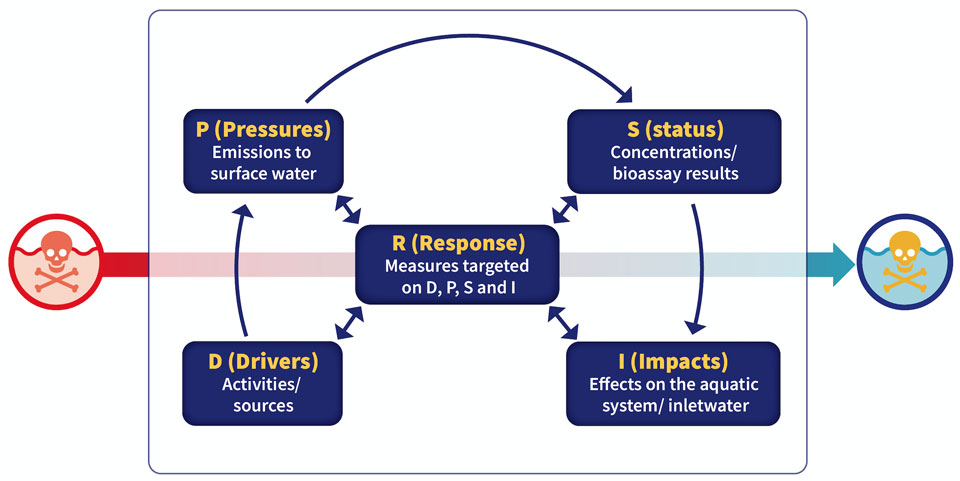
Figure 1: The DPSIR model to tackle the chemical pollution of surface water

Bioassays for unknown substances

Effect-based measurements with bioassays approach the impact of chemicals on the ecosystem by using biological material, ranging from cells to small aquatic organisms such as water fleas. With this, it is possible to detect the combined effects of all bioactive substances (known and unknown) in the water. Whole organisms react to a wide range of substances with different modes of action, whereas assays with cell lines often focus on a specific mode of action, such as endocrine disruptors.
The bioassay track tends to provide a general assessment of a location using a sampling and pre-treatment protocol, a basic set of bioassays and an interpretation tool. Basic sets for surface water and two for drinking water have been developed, which can detect substances with different toxicological effects. The interpretation tool then converts the results for each bioassay into a final score in five categories (see below).
There may be good reasons to deviate from the basic sets, e.g. if a (drinking) water authority wishes to look at a specific substance group. The selection and interpretation of such specific research requires customisation. To this end, several tools are available within Key Factor Toxicity 2 (SFT2).

From chemical substances to toxic pressure

There are several policy frameworks that focus on the assessment of individual substances. Now that the number of known substances is on the increase, it is becoming increasingly important to look at the total mixture as well. The chemistry tool is capable of translating measured concentrations into a toxic pressure of the mixture. This is carried out in three steps: 1) The input measured concentration is converted to the bioavailable concentration 2) The bioavailable concentration is converted to 'direct toxic pressure of that substance on aquatic organisms'. This toxic pressure has as its unit the potentially affected fraction (PAF) of the organisms that can live in the system. 3) The PAF for each substance is aggregated to the fraction of affected varieties for the mixture (multi-substance PAF: msPAF), for substance groups or for all substances together.

The general principle of the chemistry tool is the same as in the old ESF-TOX1, but the way in which the new tool can deal with bioavailability has been improved and the results have greater reliability. It can also be easily extended to more substances as more toxicity data become available. In addition, the Access tool from ESF-TOX1 has been replaced by an ‘R-tool’ and an interface for greater ease of use – improved access, easier data entry and clearer interpretation of the results.

Purification treatment effort

An improved water quality calculation has also been put together for the purification treatment effort (ZOI) that water companies are required to provide. When calculating the ZOI, substances are given more weighting depending on whether they exceed their drinking water target value or signalling value and whether they are harder (or easier) to treat using simple drinking water treatment techniques (Pronk et al., 2021). The higher the ZOI (the status, ‘S’ in the DPSIR model), the greater the purification treatment effort (the impact 'I' in the DPSIR model).

Interpretation of all data

What does a ZOI, bioassay score or msPAF say about the effects on drinking and surface water? This interpretation step has been greatly improved in SFT2. For both the chemistry track and the bioassay track, an interpretation method has been developed that closely follows the principles of the WFD, whereby the ‘good’ and ‘very good’ categories indicate that a system is ecologically healthy and thus needs to be protected, while the ‘moderate’, ‘insufficient’ and ‘poor’ categories call for measures that reduce toxicity (Figure 2).
The chemistry track uses a combination of the toxic pressure at the 'no effect' level (msPAF-NOEC) and the toxic pressure at the 50% effect level (msPAF-EC50). This determines which of the five categories a site is assigned to. The bioassay track uses effect signal values, i.e. the limit value at which effects on species cannot be excluded. A 'colour' is determined for each bioassay. The results are then processed in a pie chart.
A five-colour division was also created to indicate water quality in relation to the purification treatment effort – green and blue indicate that the required purification treatment effort is low enough, while with orange and red, measures are needed to reduce the effort.

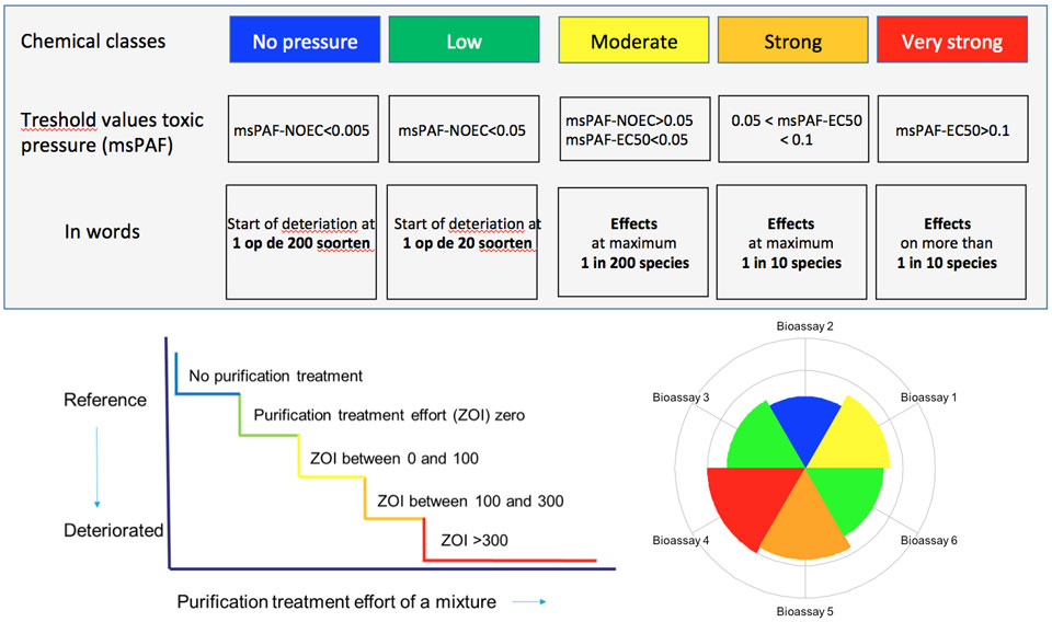
Figure 2. The elaborated quality classes for the chemistry track (above), the purification treatment effort (ZOI) and the bioassay track

Identification of sources

If the interpretation indicates that the toxic pressure needs to be reduced, the question arises as to which drivers and pressures are causing the toxic pressure. The look-up table entitled ‘Land use – substance list’ is a first step and can be used to look up the substances that may play a role for each land use. This list does not only have to be used after the fact, i.e. when the measurements have already been performed, but can also serve as a guide to determine which substances should be monitored and which specific bioassays are useful.

Conclusion

The KIWK-TOX project has delivered an approach that makes toxicity transparent and manageable. A range of tools is available on the website to help water authorities understand the threats posed by chemical pollution. The tools help companies and authorities to weigh the effects of each substance, substance group and mixture of substances.
The tools can help in the coming years in choosing measures and in monitoring the effects of measures.

Leonard Osté
(Deltares)
Wilko Verweij
(Deltares)
Sanne van den Berg
(Wageningen Environmental Research)
Paul van den Brink
(Wageningen Environmental Research)
Tessa Pronk
(KWR)
Milo de Baat
(KWR)
Leo Posthuma
(RIVM)
Inge van Driezum
(RIVM)

Summary

As part of the Knowledge Impulse for Water Quality, the Ecological Key Factor Toxicity 1 (ESF-TOX1) has been further developed into the Key Factor Toxicity 2 (SFT2). This offers water authorities and drinking water firms an improved method for getting to grips with the increasing number of chemical substances in surface water. Three important improvements have been made:

firstly, an improvement to the chemistry tool, making it more user friendly – the tool translates concentrations of chemical substances into a toxic pressure. A framework has also been introduced that further quantifies the purification treatment effort required for the production of drinking water.

The second improvement is in the bioassay track, including a renewed basic set of bioassays with associated interpretation tool for general assessment and specific bioassays for specialist research.

The third improvement concerns interpretation. The results of the chemistry and bioassay track have been developed into a classification to one of five categories, similar to those of the Water Framework Directive: none, low, moderate, high and very high toxicity.

References

R. van der Oost, L. Posthuma, D. de Zwart, J. Postma en L. Osté, 2016. Microverontreinigingen: hoe kun je ecologische risico’s in water bepalen? ESF Toxiciteit. Water Matters 2016.

Lemm, JU, M Venohr, L Globevnik, K Stefanidis, Y Panagopoulos, J. van Gils, L. Posthuma, P. Kristensen, C.K. Feld, J. Mahnkopf, D. Hering, S. Birk, 2021. Multiple stressors determine river ecological status at the European scale: Towards an integrated understanding of river status deterioration. Global Change Biology 27 (9), 1962-1975.

L Posthuma, MC Zijp, D De Zwart, D Van de Meent, L. Globevnik, M. Koprivsek, A. Focks, J. Van Gils, S. Birk. Chemical pollution imposes limitations to the ecological status of European surface waters. Scientific reports 2020, vol.10, p.1-12.

T.E. Pronk, R. C. H. M. Hofman-Caris, D. Vries, S. A. E. Kools, T. L. ter Laak, G. J. Stroomberg; A water quality index for the removal requirement and purification treatment effort of micropollutants. Water Supply 1 February 2021; 21 (1): 128–145. doi: https://doi.org/10.2166/ws.2020.289

Schuijt, L.M., F-J. Peng, S.J.P. van den Berg, M.M.L. Dingemans and P.J. Van den Brink (2021). Ecotoxicological tests for assessing impacts of chemical stress to aquatic ecosystems: facts, challenges, and future. Science of the Total Environment. 795: 148776.

^ Back to start

CO₂ reduction and resource recovery thanks to cooperation between slaughterhouse and wastewater treatment plant

Water authorities are striving to reduce CO₂ emissions and to increase resource recovery in the treatment of wastewater. Nereda technology offers energy-efficient treatment and allows a biopolymer (kaumera) to be extracted from the sludge. The Vallei and Veluwe water authority has a Nereda system at its Epe wastewater treatment plant. The wastewater treatment plant (wwtp) is currently only being used at around 60% of its capacity. As a result, it works less efficiently, leading to relatively lower production of kaumera (a biopolymer which can be recovered from granular sludge which grows in Nereda systems) and a higher specific energy consumption, and thus to higher CO₂ emissions. How can things be improved?

In 2019, consultations with a slaughterhouse near the Epe plant gave rise to a joint study into the reduced pre-treatment of slaughterhouse wastewater before discharge into the sewer. The load on the treatment plant would then be higher (more efficient) and the slaughterhouse would use fewer chemicals (iron chloride and caustic soda). The question was how the Nereda system would respond to the increased supply and different composition of wastewater (with higher concentrations of undissolved components), and what the effect would be on (net) CO₂ emissions. Pre-treatment at the slaughterhouse was turned off for 4 months, and operation of the Nereda system was intensively monitored. This article describes and discusses the results of this practical test.

Situation map

The current situation at the Epe wastewater treatment plant is shown in Figure 1.

Figure 1. Outline of the normal situation at the Epe wastewater treatment plant. The slaughterhouse wastewater is pre-treated in the Dissolved Air Flotation (DAF) system at the slaughterhouse and then enters the sewer at the wastewater treatment plant (Nereda system).

The slaughterhouse wastewater (around 300 m³/d) has a chemical oxygen demand (COD, a measure of the amount of biodegradable substances in the water) of 5 to 10 g/l. The nitrogen content is approximately 700 mg/l. In the existing situation, this wastewater is pre-treated by the slaughterhouse in a Dissolved Air Flotation (DAF) system and then discharged into the sewer. The DAF system and the Nereda system together produce 23,000 tonnes of sludge annually (1,150 tonnes dry matter/y). This is transported to sludge digesters operated by the water authority.

The experiment

The DAF plant was switched off for four months (March to June 2019). The wastewater from the slaughterhouse was discharged untreated into the sewer and then treated at the Epe wwtp (Nereda system). The Nereda system was monitored with automated measurements in the reactors and through weekly sampling. Researchers from TU Delft tracked the enzyme activity (lipase and protease) in the different (granular) fractions in the sludge.

Functioning of the wwtp

Despite an influent load that was around 60% higher, the effluent quality in both periods was comparable (Table 1) and well within the discharge norms. The downstream sand filter for extensive phosphate removal did use considerably more aluminium chloride than in the same period a year earlier: 173 l/d instead of 83 l/d, which was more than double. The phosphate load in the influent during the trial was, however, 81% higher than in the reference situation. If this is included, the relative increase in aluminium consumption is limited, at around 10% (i.e. from 0.20 mol Al/mol P to 0.22 mol Al/mol P). Phosphate removal rose from 37 to 67 kg P/day.

Table 1: The (total) influent load and average effluent composition at the Epe wastewater treatment plant during the trial and in the same period a year earlier.
*The phosphate standard of 0.3 mg/l applies from 1 April to 30 September.

Sludge production in the Nereda system increased by around 40% during the test period compared with the months before. A change in sludge production should actually be considered over a whole year as it varies with the water temperature in a treatment plant. But, if we take the usual assumption that sludge production increases proportionally to the increase in pollution unit load, and we also include the increase in aluminium consumption at the sand filter, this amounts to a sludge increase of 398 tonnes of dry matter (DS)/y. Since the DAF system at the slaughterhouse no longer produces flotation sludge, thus saving 600 t DS/y, net sludge production would decrease by around 200 t DS/y when the DAF is out of operation.

A Nereda system forms sludge granules instead of flakes, which means that the sludge settles more easily and quickly. In our experiment, the sludge changed in terms of granular fraction and settling capacity due to the higher concentration of biodegradable COD in the wastewater. At the end of the trial period, the sludge content had increased from 5.8 to 8.3 g/l and the granular fraction in the sludge (sludge particles > 0.2 mm) from 77% to 85%. Sludge growth was therefore found to be mainly caused by granular growth, with 50% of the granules larger than 2 mm. The fact that granule formation increased despite a higher concentration of undissolved constituents in the wastewater (average of 633 mg/l instead of around 317 mg/l) confirms that granular growth is quite possible with relatively high suspended solid contents. A publication by TU Delft on this full scale test investigates this in more detail. The growth of granules on wastewater with high suspended solids is known from industrial wastewater treatment in Nereda systems.

Fat accumulation

The system functioned well during the test period, but operators identified accumulation in the fat trap at the plant, deposited by the industrial wastewater from the slaughterhouse. Fat accumulation can lead to fouling and clogging and regular removal of the captured fat requires considerable effort on the part of operators. No negative effects of fat on sludge quality have been observed.

Reduced CO₂ emissions

In order to estimate the effect on CO₂ emissions of less extensive pre-treatment at the slaughterhouse, the CO₂ emissions at the slaughterhouse and at the wwtp were examined. In view of the risk of fat accumulation in the sewage system and in the receiving area of the wwtp, a scenario was assumed for this calculation in which the DAF system uses only polymer dosing and no ferric chloride and sodium hydroxide dosing. Around 50% COD would then be removed instead of the current 85%. The CO₂ emissions were calculated based on key figures from STOWA and from the Climate Monitor for water authorities.

Table 2. CO₂ emissions from the wastewater treatment plant and DAF system in the current and potential future situation

The calculation (Table 2) shows that the CO₂ emissions of the wwtp and the slaughterhouse together decrease by 75 tonnes CO₂ per year, which is a 9% reduction. This is mainly due to the fact that iron chloride and caustic soda are no longer used at the DAF system and that less sludge is transported. This more than compensates for the increase in energy consumption at the plant and the lower yield from the CHP (combined heat and power unit that produces electricity from biogas after sludge digestion), even at the lower load.

Kaumera

A demonstration system for the extraction of kaumera from aerobic granular sludge is also in operation at the Epe plant. At the end of the full scale test, kaumera was extracted from a sludge sample from the Nereda system. The yield was around 25% of the organic matter in this sludge. This is comparable with the yield when the wastewater from the slaughter house was pre-treated in the old way. Since less pre-treatment of wastewater from the slaughterhouse leads to more sludge growth in the wwtp, there is the potential to recover more kaumera. If the DAF is operated at 50% COD removal instead of 85% COD removal, Epe would produce around 30% more kaumera. Depending on how it is applied (biostimulant, coating in fertilisers, etc.), additional CO₂ savings can be achieved in the overall cycle.

Conclusions

The higher load of untreated slaughterhouse wastewater to the Nereda system at the Epe plant results in permanently high effluent quality. The sludge content in the reactors increased from 5.8 g DS/l to 8.3 g DS/l, 88% of which was due to the growth of granular sludge. A doubled concentration of undissolved constituents in the wastewater had no adverse effect. Fat removal at the slaughterhouse remained necessary. By increasing the sludge production, there is the potential to extract 30% more kaumera. A CO₂ reduction of 75 tonnes CO₂/year in Epe’s wastewater chain would also be achieved.

How to proceed?

The water authority is currently considering the continuation of the calculated scenario (50% COD removal at DAF system, without ferric chloride and sodium hydroxide dosing). This optimises the load on the wwtp and reduces CO₂ emissions in the wastewater chain. The demonstration system for kaumera extraction was built for three years of operational use, although the water authority is exploring whether production can be expanded and the plant kept in use for longer.
Many water authorities have to deal with under-loaded wastewater treatment plants. There are undoubtedly similar opportunities for CO₂ reduction by better coordinating the treatment of industrial and domestic wastewater.

Mathijs Oosterhuis
(Royal HaskoningDHV)
Erik van den Berg
(Vallei and Veluwe water authority)
Hedzer Gietema
(Vallei and Veluwe water authority)

Summary

The Nereda system at the Epe wastewater treatment plant is under-loaded. As a result, it functions with reduced energy efficiency and cannot use its full production capacity for kaumera. The water authority, Royal HaskoningDHV and TU-Delft investigated the effects of a higher load, namely with untreated wastewater from a nearby slaughterhouse. This appears to give rise to permanently high effluent quality and a significantly higher sludge content in the Nereda reactor. The latter is almost 90% due to the growth of granular sludge.

In the experiment, pre-treatment of the slaughterhouse wastewater was switched off completely. But, because of the risk of fat accumulating in the sewer and at the plant, fat removal at the slaughterhouse remained necessary. If the slaughterhouse were to pre-treat its wastewater to a limited extent, with no use of iron chloride and sodium hydroxide, a CO₂ reduction of around 75 tonnes per year could be achieved.

This article demonstrates that there are opportunities for CO₂ reduction by better coordinating the treatment of industrial and domestic wastewater. A prerequisite is of course that there is sufficient treatment capacity at the plant to cope with an increase in pollution equivalents.

References

Ortega, S. T., Pronk, M, de Kreuk, M.K., Effect of an Increased Particulate COD Load on the Aerobic Granular Sludge Process: A Full Scale Study, Processes 2021, 9, 1472. https://doi.org/10.3390/pr9081472

Kaumera Nereda Gum, STOWA report 2019-14 (Dutch)

^ Back to start

When do hydraulic engineering structures approach the end of their functional life span?

Over the next few decades, managers of hydraulic engineering structures (such as locks, pumping stations and storm-surge barriers) face a significant replacement and renovation task. Rijkswaterstaat is currently drawing up a national forecast. To create a future-proof water infrastructure, we need to answer two questions: What is the best way to intervene? When is the optimal moment? It is not only the technical and economic life cycle that counts, but the functional performance of the engineering structure as well. How do you determine that?

A structure can reach the end of its life for a number of reasons. Thus far, we have looked mainly at the development of strength degradation (technical life span) and costs (economic life span) over time. But a structure that is technically still functional and has not yet been written off can sometimes no longer fulfil its function. It then reaches the end of its functional life span, e.g. due to changes in climate, use or policy. The floods in Limburg this summer, for example, show that we will need to take more intense rainfall into account in the future, and therefore higher discharges into the tributaries and the Meuse. In order to determine the functional life span of hydraulic civil engineering structures, the Wet Civil Engineering Structures Knowledge Programme has developed the Functional Life Cycle Methodology (MFL).

Functional Life Cycle Methodology

The MFL is still under development. The aim is to obtain a generic, practically applicable methodology for mapping the end of the functional life of a structure as part of the water system. An MFL-LIGHT assessment firstly filters qualitatively those functions that are most sensitive to expected developments – i.e. aspects such as climate change, changing transport demand and changing policies. Depending on the aspect being queried, more quantitative (time-consuming) analyses of the functional life span can then be carried out in a targeted manner (MFL-MEDIUM with available model calculations and MFL-HEAVY with new model calculations). These may be, for example, analyses to identify bottlenecks for shipping or in the discharge capacity.

The MFL-LIGHT assessment has now been successfully applied in three studies, according to the water authorities that have worked with this method: 1) Climate stress test of engineering structures in the main water system, 2) Weurt-Heumen regional analysis, and 3) Proof of concept for two cases in support of the national replacement and renovation programmes operated by Rijkswaterstaat. We explain the qualitative approach below, with highlights from the replacement and renovation programme.

Figure 1. Functional Life Cycle Methodology schematic

‘Meuse’ case study: proof of concept MFL-LIGHT

Rijkswaterstaat is working on a national forecast for the replacement and renovation of hydraulic engineering structures. To support this forecast, we applied the MFL-LIGHT assessment in a proof of concept for the ‘Meuse’ river system. The aim of this assessment was to estimate the end of the functional life span of the most critical functions within the system, in order to create a comparison with the estimated technical life span. The first step of the method consists of a situation outline of the structures and networks that they are a part of. The next step is to map the associated core tasks and functions for each object group (a group of the same types of engineering structure, e.g. ‘locks’). Then, based on expert knowledge, the sensitivity of these functions to ‘drivers’ is then looked at – future developments such as climate change, transport demand and changing policies.

In the method, an object group (= group of the same types of structure) for each function is given a sensitivity score per driver. A structure or sub-task can, therefore, have several sensitivities. The values of the sensitivity score (colour coded) are defined under Figure 2. This figure is an (abbreviated) illustration of how the method works. We have based the climate drivers on the upper limit of the Delta scenarios, the WARM2050 scenario. This scenario assumes more river supply in winter, less supply in summer, warmer summers and a limited increase in transport demand. Furthermore, we assume that the shipping class of the Juliana Canal will remain unchanged (it will remain a ‘Vb corridor’). The table for the Meuse was completed by regional experts working in water management and engineering structures.

Figure 2. Development of MFL-LIGHT for the Meuse (abbreviated version).

In the case of the Meuse River, four critical object-group-function-driver combinations stand out (red and orange blocks). One of these is the combination: locks in shipping lane – facilitating shipping traffic – decrease in river discharge in summer. It has a sensitivity score of -3. After all, as river discharge decreases in summer, low water will occur more often, causing more frequent lock restrictions, which will result in longer waiting times for shipping.
The outcome of the MFL-LIGHT assessment provides insight into the most important functions that will be under pressure in the future due to (climate) change.

‘Meuse’ case study: MFL-MEDIUM

The critical object group-function-driver combinations were then worked out in an MFL-MEDIUM assessment. The remaining life span of the structure was taken into account. On the basis of a literature study and interviews with experts, the function requirement was first made specific: at what threshold does the function no longer meet the requirements and how often may this occur? We then looked for a simple relationship between driver and function.

Figure 3 shows the results for the Meuse. Due to uncertainties in the Delta scenarios, we give a range here instead of a single point in time. The figure shows that the fixed bridges and locks in the shipping lane in particular limit the functional life span of this system. The fixed bridges are already in need of intervention, while the functioning of the locks in the shipping lane is expected to require intervention in 2030. However, it is not always possible to find simple relationships, and sometimes the information is simply not available (yet). In that case, new model calculations must be made with MFL-HEAVY.

With these results, authorities can think more precisely about possible means of intervention. More detailed analyses can indicate, for example, whether the limited clearance of a fixed bridge would be better resolved by demolition – and accommodating the road traffic via another bridge – or by replacement with a higher bridge. Both interventions have a different impact on the system and its environment. Furthermore, ‘end of functional life span’ does not necessarily mean that the object needs to be replaced in its entirety – sometimes a minor modification such as installing an additional pump may be sufficient.

Figure 3. End of functional life span range for the most important object group-function-driver combinations for the Meuse system.

Challenges and uncertainties in MFL

When interpreting the results from the MFL-LIGHT, it can sometimes be difficult to identify the functional relationship between different object groups. For example, a system requirement may be that the water level in a canal bank must be maintained within a certain range. Often, multiple structures (pump, lock or weir) contribute to maintaining that water level. Quantitative insight into this kind of cohesion within the water system is often absent.

When establishing the end of a functional life spanwith MFL-MEDIUM/HEAVY, defining the requirements or ambitions is a challenge. For example, what is the maximum permissible waiting time at locks? How much is an authority willing to invest in sticking to an ambition of no more than two days’ waiting time per year? Is the action perspective with a less stringent requirement of 10 days per year acceptable? The same question can be asked of pumps. What is the minimum required availability and reliability? And how does this relate to current performance? The current performance of structures is not always monitored.

Another challenge in determining the end of a functional life span is that simple relationships are not always available. Model calculations will have to be performed to show current performance and make forecasts about the future, and these can be time-consuming. Good model schematics, in which the coherence within the system is appropriately taken into account, are not always available. In addition, forecasts involve uncertainties. Calculating the vertices of the Delta scenarios helps to map a range for the end of functional life span. An estimate can also be made of accelerated sea level rise scenarios, such as those recently presented by the KNMI and IPCC. Focused and periodic measurement of the functional performance of the system is expected to lead to a better understanding that helps to reduce uncertainty.

Further development of MFL

The phased approach in the Functional Life Cycle Methodology has clear added value for water authorities when deciding on replacement and renovation tasks. MFL-LIGHT can be used immediately. However, not all the requisite information will be available for application of MFL-MEDIUM and MFL-HEAVY. Water authorities can contribute by collecting information on how the current structure is performing in relation to requirements and ambitions. The Hydraulic Civil Engineering Structures Knowledge Programme 2021-2024 helps to map the required (further) development of models to visualise future bottlenecks; how does the system perform under the future scenario (drivers) outlined?

Nienke Kramer
(Deltares)
Joost Breedeveld
(Deltares)
Ida de Groot-Wallast
(Deltares)
Hans van Twuiver
(Rijkswaterstaat)
Evert Jan Hamerslag
(Rijkswaterstaat)

Background picture:
Weir and lock complex in the river Meuse at Grave

Summary

In view of the design life span of a large proportion of hydraulic engineering works, water authorities expect to have to make many investment decisions concerning replacement and renovation over the next few decades. These decisions are an important moment of choice; they provide an opportunity to consider desirable changes in the (multifunctional) infrastructure with a view to the future. Within the Hydraulic Engineering Works Knowledge Programme 2017-2020, Rijkswaterstaat and Deltares have developed a methodology that takes into account the decrease in (functional) performance over time and thus estimates the functional life span. This article outlines the method using the river ‘Meuse’ system as an example.

References

Deltares, 2018, Deltascenario’s voor de 21e eeuw century (revised 2017), H.A Wolters, G.J. van den Born, E. Dammers, S. Reinhard, 2018a, Deltares, Utrecht, https://media.deltares.nl/deltascenarios/Deltascenarios_actualisering2017_hoofdrapport.pdf

Kennisprogramma Natte Kunstwerken, 2020, Kennisprogramma Natte Kunstwerken, Handleiding Toolbox Functionele Levensduur, Joost Breedeveld, Nienke Kramer, Ida de Groot-Wallast, Deltares report, December 2020, 1200741-079-HYE-0001, 56 pag. https://www.nattekunstwerkenvandetoekomst.nl/producten/relatie-object-systeem/functionele-levensduur/item101

Rijkswaterstaat, Klimaat stresstest objecten HWS – Bezien vanuit het perspectief van Ruimtelijke Adaptatie, Hidde Boonstra, v1 final, 1 May 2020

Rijkswaterstaat, Regioanalyse Vervanging en Renovatie (VenR) Weurt-Heumen: analyse van de VenR-opgave voor de sluiscomplexen Weurt en Heumen van het Maas-Waalkanaal, Version 1.0, 2020

^ Back to start

Phosphate concentrations in groundwater under Dutch farms are mostly below target value

Phosphate remains a problem for the quality of surface waters in the Netherlands. However, phosphate concentrations in groundwater receive less attention. For the first time, we investigated long-term trends in phosphate concentrations in the upper groundwater on 165 Dutch farm holdings. Target values for phosphate in groundwater, which are much higher than the quality criteria for surface water, are rarely exceeded.

Phosphorus remains a problem for the quality of surface waters in the Netherlands. Due to policy measures, the annual phosphorus surplus on fertilized agricultural soils in the Netherlands has been decreasing steadily since 1990 down to 5 kg P/ha in recent years (Fraters et al. 2020). Nevertheless, long-term application of repeated fertilization in the past has led to accumulation of phosphate in the soil, and sometimes to saturation. Phosphate on agricultural land can reach surface water mainly through leaching and erosion.
Since 2015 there must be a balance between fertilization and crop removal of phosphorus in the Netherlands. Still, since that year a small increase in the nitrogen and phosphorus soil surplus in the monitored Dutch farms was observed (Fraters et al. 2020).
The historical phosphorus surplus did result in increased phosphate contents in agricultural soils. This might eventually lead to phosphate leaching to groundwater. Phosphate does not leach easily because it can be taken up by the crop and it can bind effectively to soil components. However, there are limits to the capacity of soils to retain phosphate. In almost half of the agricultural land in the Netherlands there were indications in 2014 for a potential risk for phosphate leaching to groundwater (Schoumans and Chardon 2014).

Phosphate quality criteria

The Dutch target value for phosphate in groundwater is 0.4 mg P/liter for sandy areas and 3 mg P/liter for clay and peat areas. The Dutch threshold value for fresh groundwater is 2 mg P/liter for sand areas and is 6,9 mg P/liter for peat and clay areas (https://rvszoeksysteem.rivm.nl/Stoffen). The quality values for peat and clay areas are less strict because these soils produce phosphate upon mineralization of soil. This elevates ‘natural’ phosphate concentrations in groundwater. In the dunes near the sea and in the river clay area the concentrations in groundwater are generally above 3 mg P/liter (van Vliet et al. 2010). In the coastal zone the mineralization of peat layers also leads to high P concentrations in deep groundwater. This groundwater often contains sodium, chloride and other salts of marine origin.
For surface water, the standards are much lower because of the ecological effects of phosphate. The European Water Framework Directive surface water quality criteria of 0.09 or 0.15 mg P/liter, depending on the water type, are commonly exceeded in Dutch surface waters. The average total phosphorus concentration in agriculture specific surface waters was 0.4 mg P/liter in 2020 (Fraters et al. 2020).

Nationwide monitoring program

In the Netherlands we have a national Minerals Policy Monitoring Programme which provides information on the effects of Dutch Minerals policy on agricultural practices and water quality. The RIVM and Wageningen Economic Research cooperate to collect annual information about agricultural practices and water quality on approximately 400 Dutch farms (van Duijnen et al. 2021). For this study, we investigated the trends of phosphate concentrations in the phreatic groundwater on participating farms since 2006. On each farm, the top meter of groundwater was sampled annually from 16 freshly dug boreholes evenly distributed across the farm plots.
The participation of farmers in the monitoring program is voluntary. Each year a number of farmers leave the program and additional farms have to be selected in order to remain a representative nationwide selection of farms. In order to accurately detect trends, we have selected the 165 companies that have been participating continuously since 2006.
Since quite a number of measurements were below the detection limit of 0.013 mg P/liter, we used model calculations to estimate the average phosphate concentration on each farm.

Results

Notably, only five farms (3%) showed a significant increase and no farms showed a significant decrease in phosphate concentration over the years (Fig. 1). Significant means having a p-value with Bonferroni correction of less than 0.05.

Figure 1. the annual slope of the phosphate concentrations per farm from 2006 till 2020. The 165 farms were ordered according to the annual slope of the phosphate concentration. Most farms are on or close to the horizontal line which indicates there is no slope and therefore no increase or decrease.

Green dots indicate the three farms with a significant increasing trend (P Bonferroni value <0.05) in phosphate concentrations over the years 2006-2020. Blue dots indicate the 14 farms with no significant trend but with phosphate concentrations above 0.4 mg P/liter. The 2 red dots indicate the two farms with both an average phosphate concentration above 0.4 mg P/liter and a significant increasing trend.
Conclusion: 160 farms did not show any significant trend. Only 16 farms (14 blue and 2 red) had a phosphate concentration above 0.4 mg P/liter.

Figure 2. farms ordered with increasing phosphate concentrations from 2006 till 2020. The upper horizontal line indicates the Dutch target value for groundwater in the sand region (0.4 mg P/liter) and the lower one is the detection limit. All farms stay below the Dutch target value of 3 mg P/liter groundwater for clay and peat soils.

In figure 2 the green red and blue dots correspond with figure1. Figure 2 shows that about 90% of the farms have a mean phosphate concentration below 0.4 mg P/liter. Six farms even have a mean phosphate concentration below the detection limit of 0.013 mg P/liter.

Table 1. The correlation between the mean phosphate concentrations on the farms with a number of other elements/ions.

Table 1 shows that phosphate concentrations correlates with the sea water components chlorine, magnesium, sodium (Na) en strontium and with the electric conductivity EC which is also high in sea water. There is also a positive correlation with ammonium (NH4+), and a negative correlation with nitrate, copper and cadmium. Also, deeper groundwater has higher phosphate concentrations.

Discussion

This study shows that only a very limited percentage of farms had a positive phosphate trend in the upper groundwater. In the Netherlands the deeper groundwater contains elevated levels of seawater components like Cl, Na, Sr, Mg and the electric conductivity. We found a positive correlation between phosphate concentrations and the sea water components. In addition, a positive correlation with ammonium (NH₄⁺) was found which occurs commonly in deeper anaerobic ground water.
Deeper groundwater layers in the peat and clay regions of the Netherlands show elevated phosphate and ammonia concentrations due to the historic mineralization of peat layers (van Vliet et al., 2010). We now also observe on a few farms an increase in phosphate and ammonium concentrations in the upper groundwater. On rare occasions this will be due to phosphate coming from the soil surface but the main cause is probably the upwelling of deeper groundwater.
The phosphate concentrations in the upper groundwater in this study are in correspondence with the phosphate concentrations in the Flemish sandy region (Mabilde, De Neve, and Sleutel 2017). Our data show that even the lowest target value for phosphorus is rarely exceeded in the upper groundwater under Dutch farms. This target value is much higher than the surface water quality criteria from the European Water Framework Directive. Overfertilization with phosphorus still remains a serious problem for terrestrial and aquatic ecosystems but apparently not yet for Dutch groundwater. But as the target values for phosphate in groundwater are much higher than for surface water. it is possible that groundwater discharge through leaching or drainage leads to high phosphate concentrations in surface water.

Patrick van Beelen
(National Institute for Public Health and the Environment (RIVM))
Annemieke van der Wal
(National Institute for Public Health and the Environment (RIVM))

Summary

The Dutch Minerals Policy Monitoring Programme monitors the groundwater quality. The phosphate concentrations in the upper meter of the groundwater were lower than the target value of 0.4 mg P/liter at most of the 165 farms participating since 2006. Only five farms showed a significant increase of the phosphate concentration in groundwater while the other farms did not show any significant trend.

Acknowledgements

The authors thank the LMM monitoring team and TNO for groundwater sampling and analyses. This research was funded by the Ministry of Agriculture, Nature and Food Quality.

References

Fraters, B., A. E. J. Hooijboer, A. Vrijhoef, A. C. C. Plette, N. van Duijnhoven, J. C. Rozemeijer, M. Gosseling, C. H. G. Daatselaar, J. L. Roskam, and H. A. L. Begeman. 2020. 'Landbouwpraktijk en waterkwaliteit in Nederland; toestand (2016-2019) en trend (1992-2019) : De Nitraatrapportage 2020 met de resultaten van de monitoring van de effecten van de EU Nitraatrichtlijn actieprogramma's', RIVM rapport 2020-0121: 232.

Mabilde, L., S. De Neve, and S. Sleutel. 2017. 'Regional analysis of groundwater phosphate concentrations under acidic sandy soils: Edaphic factors and water table strongly mediate the soil P-groundwater P relation', Journal of Environmental Management, 203: 429-38.

Schoumans, O. F., and W. J. Chardon. 2014. 'Phosphate saturation degree and accumulation of phosphate in various soil types in The Netherlands', Geoderma, 237: 325-35.

Van Duijnen, R, PW Blokland, A Vrijhoef, D Fraters, GJ Doornewaard, and CHG Daatselaar. 2021. "Agricultural practices and water quality on farms registered for derogation in 2019." In Landbouwpraktijk en waterkwaliteit op landbouwbedrijven aangemeld voor derogatie in 2019. Rijksinstituut voor Volksgezondheid en Milieu.

Van Vliet, M. E., A. Vrijhoef, L. J. M. Boumans, and E. J. W. Wattel-Koekkoek. 2010. 'De kwaliteit van ondiep en middeldiep grondwater in Nederland [Quality of shallow and medium-deep groundwater in the Netherlands]', RIVM rapport 680721005

^ Back to start

Alternative water sources and decentralised water supply networks for a climate-proof water supply

The Water Nexus research programme looks for alternative water sources to achieve water self-sufficient regions. The motto of the programme is ‘salt where possible, fresh where necessary’. But which water source do you opt for and how do you get the water to users?

Zeeuws-Vlaanderen is not self-sufficient when it comes to fresh water. The groundwater is mostly brackish and the North Sea and Westerschelde are salt water bodies, so fresh water is now pumped to the area from the Biesbosch over a distance of 120 km to meet water requirements. Zeeuws-Vlaanderen is reliant on this external water supply. In times of drought, this water source (i.e. the reservoirs in the Biesbosch) may find themselves under pressure, which can lead to water shortages for residents, industry and/or agriculture. There are several alternative and renewable water sources available locally, including fresh, brackish and saline groundwater, rainwater and treated wastewater. Using these water sources could reduce dependency on the Biesbosch and make the water supply future-proof.
To use these alternative water sources, a switch to a decentralised water supply is an option – this would require large investments in new infrastructure, a complex design and complex implementation. Alternative sources must be selected, as well as the most cost-efficient way to move water to where it needs to be used.
The aim of the Water Nexus research programme is to investigate how agro-industrial regions can become self-sufficient in water, with salt water and wastewater seen as part of the solution, rather than a problem. A new tool, WaterROUTE, is helping to design new ways of supplying water and thus support decision-making. The starting point is to develop decentralised water systems that are in balance with local ecosystems. WaterROUTE visualises water availability and regional water demand with hydrological models, combined with methods of GIS and mathematical programming.

Sources in focus

The WaterROUTE tool has been tested on a case study in Zeeuws-Vlaanderen. The first step is to identify the alternative water sources with the maximum renewable water availability for each source (see Figure 1). There are 25 locations with availability of fresh groundwater and several towns and villages with rainwater and wastewater.
The availability of fresh groundwater is mapped with a 3D groundwater model linked to a salt transport model (Van Baaren et al., 2016, Willet et al., 2020). Potential fresh groundwater wells are mapped with an upper limit for salinity of 1500 mg chloride per litre. Extraction from the wells must not affect local ecosystems through salinisation or a severe drop in groundwater. We chose a maximum drop of 50 mm as the input parameter for the model (Oude Essink and Pauw, 2018). Adjustment is possible if stricter requirements prove necessary.
A total of 6.1 million m³ per year of renewable fresh to brackish groundwater is available.
In cities and villages, 4.6 million m³ of rainwater and 4.2 million m³ of wastewater could, theoretically, be collected. This is based on precipitation data from the dry year 2018, rainwater harvesting from all roofs with an efficiency of 85 per cent and decentralised wastewater treatment with a volume based on daily water consumption per inhabitant (118 litres).

Figure 1: Alternative water sources in Zeeuws-Vlaanderen and the most cost-efficient pipelines between them

Feasible pipelines

WaterROUTE then maps all possible connections between water users and water sources based on the lowest relative cost of constructing pipelines (Figure 1). Each land use (cities, natural areas and agricultural land) has different construction costs – the cost of building pipelines along existing infrastructure such as roads is, for example, lower than through cities or natural areas. The relative costs were determined in consultation with experts in the field of water distribution networks. The relative costs for different types of land use are then converted to a cost grid with GIS. The potential connections with the lowest cost are generated using a ‘least cost path algorithm’.

From water demand to a decentralised supply network

As a final step, WaterROUTE takes water demand (quantity and quality) to calculate the pipeline network that will meet that demand, based on cost minimisation. The result is an overview of the most suitable water sources.
In the optimisation, the model determines which pipelines should be used and how much water should flow through each pipe, with a piece-wise linear cost function minimised for each pipe. The cost function is based on the cost of building new pipelines and pumping costs.
For the Zeeland-Vlaanderen case study, we assumed an industrial water user in the Terneuzen region. In this article, we show the results for an annual water demand of 4 million m³. We have run the model for three scenarios: (1) Groundwater only, (2) Groundwater and rainwater and (3) Groundwater, rainwater and decentralised treated wastewater. The current situation, with supply from the Biesbosch, is not included.

More sources, smaller network

Figure 2 shows the different networks required to move the requisite amount of water to the water user. With more alternative water sources, the requisite water network would become significantly smaller:
• Scenario 1 - 100% groundwater: 63.7 kilometres of pipeline;
• Scenario 2 - 54% groundwater and 46% rainwater: 37.1 kilometres of pipeline;
• Scenario 3 - 34% groundwater, 30% rainwater and 36% treated wastewater: 23.2 kilometres of pipeline.
Compared to scenario 1, costs in scenario 2 would fall by a quarter and in scenario 3 by half. In our example, the operational costs for the pipelines are based on the energy costs for pumping (€0.2/kWh) and the investment costs depend on the required pipe diameter and the total length of the pipelines. In general, a minimum flow velocity of 0.4 m/s and a maximum flow velocity of 1.5 m/s have been assumed. (Mesman and Meerkerk, 2009). For WaterROUTE, the upper limit of 1.5 m/s is significant because after that point, pumping costs increase dramatically. The key figures that we have used for the construction of new pipelines are €50/m per 100 mm diameter – so a 300 mm pipe would cost €150/m (Willet et al., 2021).
When extracting groundwater, the operational costs concern the energy to pump the water from under the ground (€0.2/kWh) and the investment costs for drilling the wells. For each location, we have assumed a cluster of small-scale wells, where the costs depend on the depth of each well (we calculate €50/m).
In order to have the collected rainwater available all year round, we have assumed storage in open basins that are 3 metres deep. The investment costs for this comprise the costs for the earthworks and the construction of the waterproofing membrane (initial investment costs of €15,000 per basin, with costs increasing by €2.40 per m³ of realised capacity). In addition to the earthworks, we have also calculated the purchase costs for the (agricultural) land (€75,000/ha).
For wastewater, we have assumed that it is properly treated for reuse at the water treatment plant and that no additional costs are included.

Brackish water

In Zeeuws-Vlaanderen, fresh groundwater is scarce while brackish groundwater is abundant. Consequently, we have also looked into the use of brackish groundwater. In this scenario, the WaterROUTE model calculates the most suitable sources based on the maximum permissible salt concentration (fit-for-purpose water). We ran the model for moderately brackish water with maximum concentrations at the end user of 375, 400, and 425 mg chloride per litre (Willet et al, 2021). The cost of the network has been shown to decrease significantly as saltier water is mixed with fresher water closer to the water user.
The model can also be used to clarify which is cheaper: saltier water with low transport costs but high desalination costs, or fresh water with high transport costs but low desalination costs. In areas where the quality of water sources is changing due to salinisation, this functionality can be used to design water systems to be robust in the long term.

Figure 2. The cheapest WaterROUTE network and the most suitable alternative sources for an industrial water user in Terneuzen (4 million m³). Scenario 1 (top) uses only groundwater, scenario 2 (bottom left) uses groundwater and rainwater and scenario 3 (bottom right) uses groundwater, rainwater and decentralised treated wastewater. The current situation is not included.

Conclusion

Decentralised water systems with alternative water sources can offer a solution to meet the water demand of all water users in a region, and make the water supply climate-proof. The WaterROUTE tool enables research into decentralised systems and can thus facilitate design and decision-making by comparing different options (including the current one). The model can be applied to any regional water system. However, it is essential to know what alternative sources are available, what sustainability criteria apply and what costs need to be taken into account. The model can include the costs relevant to the user and can be expanded to include, inter alia, the costs of wastewater treatment or underground storage.

Koen Wetser
(WUR)
Joeri Willet
(WUR)
Huub Rijnaarts
(WUR)

Summary

Locally available alternative water sources can contribute to a climate-resilient water supply. This requires a switch to a decentralised water supply. Both the design and decision-making are, however, complex and it is difficult to properly evaluate different scenarios. With the new WaterROUTE tool, we have compared the availability of local groundwater, rainwater and wastewater for Zeeuws-Vlaanderen with the water consumption of a large industrial water user. By using more alternative water sources, the required pipeline network becomes smaller, with lower costs overall.

Sources

Mesman, G.A.M., Meerkerk, M.A., 2009. Evaluatie ontwerprichtlijnen voor distributienetten / Evaluation of draft guidelines for distribution networks KWR, 48 pp. http://api.kwrwater.nl//uploads/2017/10/KWR-09.073-Evaluatie-ontwerprichtlijnen-voor-distributienetten-vertakte-netten.pdf.

Oude Essink, G.H.P., Pauw, P.S., 2018. Evaluation and in-depth study of groundwater extraction rules in the province of Zeeland, 170 pp. https://publicwiki.deltares.nl/display/ZOETZOUT/Modelstudies (accessed 16/01/2020).

Van Baaren, et al. 2016. Verzoeting en verzilting van het grondwater in de Provincie Zeeland, Regionaal 3D model voor zoet-zout grondwater, Deltares report 1220185 / Salinisation and groundwater in the Province of Zeeland, Regional 3D model for fresh-saline groundwater, Deltares report 1220185, 86 pp. https://publicwiki.deltares.nl/download/attachments/55640066/1220185-000-BGS-0003-r-Verzoeting%20en%20verzilting%20freatisch%20grondwater%20in%20de%20Provincie%20Zeeland-def.pdf?version=1&modificationDate=1490345125944&api=v2 (accessed 27/05/2021).

Willet, J. et al. 2020. Water supply network model for sustainable industrial resource use a case study of Zeeuws-Vlaanderen in the Netherlands. Water Resources and Industry 24, 100131.

Willet, J. et al., 2021. WaterROUTE: a model for cost optimization of industrial water supply networks when using water resources with varying salinity. Water research, 117390.

^ Back to start

Eight nitrate sensors compared, what are the differences?

There is little information on the reliability of sensor readings. A measurement campaign compares eight different types of nitrate sensors.

In the Netherlands, the standards of the European Water Framework Directive for surface water are not yet achieved everywhere. Many of the excess values are caused by excessively high concentrations of nutrients in surface water, such as nitrogen and phosphorus. The concentration of nutrients in surface water has high temporal variation. The composition of the water changes constantly depending on sunlight, water temperature, precipitation and agricultural activities.
Monthly conventional measurements are by definition snapshots, and the great dynamics in the concentrations remain hidden. This does not pose a problem to a large national or regional monitoring network. Thanks to the large number of measurements, a reliable national or regional average can be determined in spite of the variations.
But, for a reliable picture of water quality at one specific location, for example in a farm ditch, monthly snapshots are insufficient. The average becomes more reliable if more measurements are taken. High-frequency measurement of water quality with sensors has, therefore, great promise. Sensors make short-term variations in water quality visible. With this, very accurate loads and average concentrations can then be determined. Moreover, high-frequency measurements provide a great deal of insight into the most important transport processes. Sensor measurements show when nutrient losses occur, which can help with policy formulation and evaluation.
Sensors are not available for all nutrients. Phosphate and ammonium, for example, are not easy to measure with sensors. For nitrate, the options are somewhat wider – there are three types of sensor available on the market and many sensor suppliers offer their own brand of sensor.
However, researchers starting out with sensors are often completely unclear on how accurately sensors measure and which sensor is most suitable for which application. No comparative research is available and researchers tend to report only successes, not failures. A measurement campaign was carried out to look at how the accuracy of nitrate sensors compares amongst the sensors themselves, and with laboratory measurements.

Design of the measurement campaign

This measurement campaign was established within the WaterSNIP Participant Group. WaterSNIP is an acronym for Water Sensors Nutrients Innovation Programme and is an innovation programme of the Minerals Policy Monitoring Programme (LMM). By deploying sensor technology, the RIVM hopes to make the LMM more efficient and future-proof.
The campaign was carried out between early October and early December 2020 at the Rijkswaterstaat measuring station in the Meuse near Eijsden (Photo). The highest nitrate concentration was expected during this period, as nitrate leaching occurs in autumn.
A total of 8 sensor suppliers and developers from the WaterSNIP Participant Group participated in the measurement campaign. They did this free of charge; the entire campaign was carried out with a ‘closed-circuit system’ (see Table 1). The participants were not recruited either, everyone volunteered after a webinar in which this idea was suggested.

Table 1: Participants in the measurement campaign with nitrate sensors

Measurement techniques for nitrate sensors

There are three types of sensor on the market for measuring high-frequency nitrate, the Ion-selective electrode (ISE), the UV method and the wet-chemical method. The ISE measurement is based on an electrical potential difference between the ISE and a reference electrode. Between the water to be measured and the ISE is a membrane that ensures the specific reaction to the ion to be measured, in this case nitrate.
UV sensors work with a UV light source and a receiving sensor for UV light sent through a water sample. The nitrate present in the water absorbs a specific part of the UV light. The nitrate concentration is therefore determined by the degree of absorption of a specific part of the UV-wave spectrum.
The wet-chemical auto analysers use reagents that trigger a colour reaction depending on the concentration of the parameter being measured. The colour change is measured with a spectrophotometric sensor.
One ISE, one autoanalyser and six different types of UV sensor participated in the measurement campaign. The measurements with the ISE deviated so much from the other measurements due to malfunctions that the participant withdrew from the measurement campaign.
The water quality of the Meuse was relatively stable during the measurement period. In order to test the sensors under heavily varying conditions as well, the sensors were placed in a reservoir at the measuring station after the Meuse experiment, in which three additional experiments were carried out:

- The nitrate concentration in demineralised water was incrementally increased from almost 0 to 140 mg/l in order to test the measuring range for nitrate;
- The chloride concentration was increased from Meuse water to slightly brackish conditions to investigate the influence of chloride on the nitrate measurements;
- The reservoir was filled with tap water and nothing was done for one day and one night to investigate the measurement stability and the influence of temperature.

Results of the experiments

Meuse water, two months
The experiment with the sensors in the Meuse shows that the variation in nitrate concentration is properly picked up by all sensors. The pattern of peaks and troughs is recorded identically by the sensors. The height of the measured nitrate concentration of the sensors deviates (see Figure 1A). The difference between the sensor with the highest measurement and the sensor with lowest measurement is around 4 mg/l. This deviation is probably due to the calibration of the sensors. Most sensors are calibrated on a calibration liquid or measure with factory settings. The composition of the water in the Meuse is different to the calibration liquids, which can lead to deviations during calibration. It would be best to calibrate the sensors to the actual nitrate concentration in the Meuse. This can only be done once the results of a number of laboratory analyses are known. In view of the uncertainty of laboratory analyses (plus and minus approx. 1 mg/l, or approx. 10%), it is advisable to use several measurements.

Figure 1 A. All nitrate measurements in the test. The horizontal lines indicate the beginning of the sensor measurements (sensors are not positioned at the same time). The sensor measurements show that the pattern of nitrate concentration is similar, but that the level of concentration differs. B. The corrected nitrate concentrations.

In this experiment, we corrected sensors retrospectively for the first three laboratory measurements. The average difference between the laboratory measurements and the sensor measurements was calculated at these times. This difference was used as a fixed correction value for the whole two-month series of the Meuse water experiment. An additional correction was applied to the auto-analyser, as the settings were adjusted at the beginning of November.
After applying the correction, the sensors measure water quality very synchronously and the measured nitrate concentration is almost the same over the entire measuring period (see Figure 1 B). After around one month of measurement, from the beginning of November, the sensors do seem to show some difference. The increasing deviation of sensors from the 'true' concentration is called drift and can be caused by contamination of the sensor. Cleaning and/or recalibration are then recommended.

Additional experiments
The experiments in the reservoir also provide valuable information concerning the operation of the sensors. After increasing the nitrate concentrations, the measurements from the sensors appear to be very different (see Figure 2). The reason for this is that the sensors are set to a certain expected concentration. The sensors that were set to a lower concentration have a deviation at higher concentrations.
It is noteworthy that the laboratory measurements also came out well below expectations. No explanation has been found for these anomalous measurements; we suspect that errors were made somewhere in the analysis process.
The experiment with heavily increased chloride concentrations shows that the UV sensors are not sensitive to chloride. Chloride does not interfere with UV measurement. However, the auto-analyser does show a deviation at high chloride concentrations.
In the last experiment, a changing temperature for some sensors shows a very small deviation in the measurement. It is, therefore, possible that the increased variation in Figure 1B is an effect of changing temperature. During the Meuse water experiment, the temperature dropped by around 7 degrees. However, it is not possible to determine which sensor deviates. The laboratory measurements are not sufficiently accurate for this.


Figure 2. The measurements during the nitrate experiment, plotted against the expected nitrate concentration.

Conclusions

The measurement campaign shows that if a nitrate sensor (UV method or auto-analyser) is properly calibrated, the measurement is more accurate than the laboratory measurement. Moreover, the continuous determination allows much better determination of the change in nitrate concentration (the dynamics). This provides insight into the processes that lead to nitrate leaching, and thus a more accurate average of nitrate concentration can be determined.
Temperature and chloride have little influence on the measured value. The differences between the sensors are mainly determined by the initial calibration of the sensors. It is, therefore, impossible to say which sensor is ‘best in the test’; all sensors tested can be used to measure variations in nitrate concentration.

Arno Hooijboer
(RIVM)
Elma Tenner
(RIVM)
Joachim Rozemeijer
(Deltares)

Background picture:
The Meuse near Eijsden as seen from the measuring platform. Most sensors are attached to the railing and placed directly in the Meuse.

Summary

More and more water authorities are using sensors to determine water quality at high frequencies, but there is little information on the reliability of sensor measurements. In this measurement campaign, eight different types of nitrate sensor were compared on the Rijkswaterstaat measuring platform in the Meuse near Eijsden.

^ Back to start

Fish migration research automated

Fish travel great distances. As they do, they often become stuck on pumping stations, weirs and locks. Sound knowledge is required in order to be able to identify bottlenecks to fish migration and to tackle them one step at a time. Fish move 'under the radar', so research is complex and time-consuming. Using a monitoring module, automated with the latest techniques, Vislift and RAVON wish to accelerate research into fish migration. This article describes the first trial of the module, aimed at glass eels.

Fish use different habitats for different life stages – to reproduce or grow, for example. In the Netherlands, there are more 60,000 obstacles along their swimming routes, including pumping stations and weirs. Considerable attention is paid to identifying bottlenecks to fish migration in order to tackle them one step at a time. In many cases, this looks at where fish are ‘in the queue’ and how easily they can enter. But, more detailed knowledge is needed to resolve bottlenecks properly. Young eels (glass eels), for example, swim at night, so many of their movements remain unseen. How can we learn more about the natural migratory behaviour of fish? And do that with a minimum of labour? Vislift and RAVON combined their technical and ecological knowledge and jointly designed a completely new monitoring module, focused on inland migration. The aim was to automatically detect glass eels and other species, to determine their activity and supply and help understand them.

First trial: Zierikzee

The first use of the monitoring module was aimed at glass eels and took place at polder pumping station 't Sas in Zierikzee. The pumping station discharges fresh to brackish water into the salty Oosterschelde. To put it simply, the monitoring module is a container in which fish can swim in and out, oriented towards an attraction flow (fresh water, supplied from the other side of the pumping station via a hose). Glass eels can remain inside the module for lengthy periods as it is fitted with brushes between which the eels can rest. In addition, there is a freely movable swim opening, camera monitoring, a fish counter and various water quality sensors. The data arrive online in real time to a single portal, with automatic image recognition through machine learning. With this, every fish that swims past the camera into or out of the module is registered and automatically identified by species. Subcutaneous colour tags or ‘VIE tags’ (Visible Implant Elastomer Tag) were used to correct double counting and gain insight into the local glass eel population and catch efficiency. A total of 147 marked glass eels were released outside the module and 60 with a different colour code were released as a control group inside the module.

Three measurement periods

During the first ten-day period after release (P1), the entrance had a maximum attraction flow of 42 cm/s at 1.78 m3/min. The tagged glass eels in the module were counted on days 3, 6 and 9, and then kept in a live tank.
At the beginning of the second period (P2), the control group was returned to the module. The remaining specimens caught during P1 were released and after 8 days, another manual count was carried out to identify double counting. During this second period, the pump ran at half speed to see the effect of a weaker attraction flow (21 cm/s at 0.92 m3/min).
As the intake was lower than in P1, the attraction flow for P3 was set to 100% again, to verify the results of P1. Unfortunately, during P3, the power supply was interrupted for 6 of the 9 days.
Due to the large number of fish entering and accumulating in the module, all glass eels were repeatedly released outside the module after being counted.

Results

The automatic image recognition system recorded a total of 80,045 fish passing in front of the camera: primarily glass eels (73.4%), followed by three-spined stickleback (21.0%), herring (4.4%), older stages of eel (1.1%), flounder (0.1%) and a single observation of ten-spined stickleback.

Of the glass eel movements, 78% were recorded between sunset and sunrise (Figure 1). There was a significant effect of tide: low tide gave more registrations than high tide (p<0.001) and ebb tide (p<0.001).
Figure 1. Glass eel recordings over 24 hours and by tide

In the first measurement period (P1), 63% of marked glass eels were in the module within 3 days of release (Figure 2). The intake curve then flattens out to over 76% (112 out of 147 glass eels) after 10 days. In the second period, with the weaker attraction flow, the intake efficiency was considerably lower: 39% in 8 days. After resetting the pump to 100%, 65% of the marked glass eels were in the module after 9 days (despite the power failure). The flattening of the curve in Figure 2 means that every 24 hours, 10.3% of the glass eel population stopped migrating, e.g. due to departure or death. Of the remaining supply, 37.5% entered the monitoring module every 24 hours. Approximately 8% of the control group left the module each day; therefore, the length of stay was high. Many returned over the following days.
Figure 2. Efficiency of the monitoring module over three periods. During P1, glass eels from the VIE tag groups (n=10) in the module were counted after 3, 6 and 10 days (mean and standard deviation). The trend line based on P1 leads to a population model in which 10.3% stop local migration every day and 37.5% of the remaining population migrate into the module.

Due to the high capture efficiency and repeated release and return swimming, a large proportion of glass eels were observed several times. Using the VIE tags, catches and re-catches, it is possible to calculate relative numbers and a 'snapshot' of the present population. On day 1 of P1, 147 glass eels were marked with a VIE tag and released into the research area, on day 3, 779 glass eels were taken from the module, of which 94 of the 147 released. The total population (marked and unmarked) is therefore 779x147:94 = 1,214 glass eels (with a binomial 95% confidence interval of 1,062-1,351). This is not, of course, the total glass eel arrival throughout the season; due to influx and outflux, the total arrival is actually higher. Volunteers caught 104 glass eels with a dip net throughout the migration season. From the number of marked eels, it can be deduced that this is approximately 2% of the total recruitment, which can therefore be calculated at 4,367 (with a considerable margin: 95% Poisson BI 1.931-8.606).

Comparison of the automated and manual counts of the influx into the module made it clear that not all colour codes were equally detectable. With blue light instead of neutral light, this improved from 37% to 68%.

Discussion and conclusion

The module dovetails well with the inland migration behaviour of glass eels (and other species). After all, a considerable number of fish, particularly glass eels, swim into the monitoring module with the polder water attraction flow. This can provide considerable new knowledge. For glass eels, over 76% of the marked specimens visited the module in 10 days, we consider this to be representative of the local supply. An optimal attraction flow rate and flow rate have not yet been found; more settings need to be tested for this. Automatic image recognition makes it possible to understand migration activity. At the research site, activity peaks are during the night and low tides, possibly triggered by fresh water leaks from the polder.
Fish swim back and forth and are detected several times. Image recognition still needs to be refined in order to determine the 'net' number of fish swimming by more precisely (automatically). The automatic recognition of VIE tag colours is also not yet conclusive. Use of VIE tags is essential to quantify supply, correct for double counting and derive population models.
Furthermore, a large number of glass eels accumulated in the module due to the high intake and time spent in the module. This made periodic manual emptying necessary. In order for the module to function fully autonomously, a solution must be found for this – e.g. by automatically releasing the fish at the location or perhaps behind the pumping station.

Applicability and further development

In its current form, the module improves the options for researching fish supply and activity at potential fish migration bottlenecks. Prior to the construction of a fish passage, it is possible to test a number of specifications, such as flow velocity, flow rate, location and positioning of the attraction flow. Further fine-tuning of gross and net migration movements would make it possible to calculate automatically with absolute numbers. In a follow-up project, the automatic VIE tag recognition will be further developed: the input of more image material will improve the reliability of detections through the learning ability of the algorithms. If accumulation can be prevented, manual emptying will become unnecessary and the module will be able to operate fully autonomously. VIE tagging of different groups of glass eel or other species would be the only manual work remaining.

Martijn Schiphouwer
(RAVON)
Anne Regtien
(Vislift)
John van Boxel
(Vislift)
Sanne Ploegaert
(RAVON)

Background picture:
Monitoring module at polder pumping station 't Sas in Zierikzee

Summary

Continuous monitoring of fish with variable conditions (such as attraction flow rate) provides deeper insight into migration and behavioural patterns. Automatic species recognition contributes to the efficient collection of large amounts of detailed data. The monitoring module, designed with new techniques and variable settings, has proven itself capable of investigating migrating glass eels and other species. When applied in Zierikzee, aimed at glass eels, 63% of the glass eels present visited the module within 3 days; after 10 days this increased to more than 76%. Most glass eel activity (78%) was observed between sunset and sunrise. There were also significantly more registrations at low tide than at high or ebb tide. VIE tags are necessary for quantification – in this case, a present population was identified in the order of 1,200 specimens. Automatic VIE tag recognition is not yet conclusive and will be further developed in time to come.

Acknowledgements

We would like to thank Waterschap Scheldestromen for allowing us to use the facilities at the 't Sas pumping station. We would also like to thank participants in the National Postcode Lottery for their contribution to Red Onze Paling, which made it possible for RAVON to invest in this project. We owe the knowledge base from the Samen voor de Aal (‘Together for the Eel’) cross-net monitoring to the volunteers at Team Sas.

References

Kooiman, M. & Ploegaert, S.M.A., 2020. Samen voor de Aal; Kruisnetmonitoring Zeeland 2017-2020. Projectnummer 2020.031. Stichting RAVON, Nijmegen.

Schiphouwer, M.E. & Kooiman, M, 2021. Landinwaartse migratie van aal via de Noord-Hollandse IJsselmeerkust. Onderzoek naar intrek, aanbod en knelpunten. RAVON, Nijmegen. Rapportnummer 2019.053.

^ Back to start

New lab method to predict sludge dewatering at wastewater treatment plants

Dewatering and processing sewage sludge is a major cost item for water authorities. However, research to improve this is difficult because the current lab scale dewatering methods are very different from those used at wastewater treatment plants. Now a simple lab method is available with two advantages: both its mechanism and the results are comparable with dewatering installations at sewage plants, which makes the method predictive of practice.

In the Netherlands, the water authorities produce 1.3 million tons of dewatered sewage sludge annually. The dewatering and handling of sewage sludge are expensive and can account for as much as 20-30% of the operational cost yearly. Transportation of dewatered sludge can cost 5 to 10 euro per ton of sludge and the costs of final disposal can be as high as 75 to 100 euros per ton of sludge. Doing experimental tests with a full-scale dewatering installation to improve sludge dewatering is not easy, because the equipment is needed to process the sludge continuously and fast switching of settings is not possible. Moreover, laboratory research on dewatering was often debatable because of the discrepancy with the situation at wastewater treatment plants. Therefore, there was a need for a new method which makes laboratory research valid again.

Laboratory and practice

There are different laboratory-scale methods to evaluate dewaterability and the effect of sludge pre-treatment on dewaterability. Examples are the CST-test ('capillary suction time') and the SRF-test ('specific resistance to filtration'); the binding energy test (determination of the required energy to remove the water from sludge floc). However, with these methods it is not possible to predict the dry matter content (%DS) of the sludge cake of full-scale dewatering installations. Moreover, all these tests work in a totally different way compared to full scale plants. For example, the commonly used CST and SRF tests are based on gravity and mild vacuum respectively, while in the full scale a mechanical force removes the water from the sludge structure. Another drawback is that these tests can only report the filterability of the sludge in terms of time: the higher the filtration time, the less the dewaterability of the sludge. However: in practice, there is no relation between the time and dry matter content of the sludge cake.

Discrepancies

The results of studies by different laboratories are often not very comparable. For example, Zhang et al. (2019) determined the bond energy of sludge, which is the required energy to remove water from sludge matrix, to investigate the effect of anaerobic digestion on sludge dewaterability. The researchers concluded that dewaterability improved with anaerobic digestion, based on the measured lower binding energy values. However, Liu et al. (2021) came to an opposite conclusion based on CST values. They observed that anaerobic digestion increased the CST values of sludge from 70 s to 1400 s and concluded that the dewaterability deteriorated after anaerobic digestion. The results of these studies are clearly contradictory and therefore have no predictive value for full-scale wastewater treatment plants.
In the past, testing of dewaterability in laboratories was often done with a mini-filter press, for example, a Mareco mini filter press. However, in recent years this method has proven less reliable due to changes in sludge composition as a result of bio-P sludge and/or the application of heat pre-treatment. Due to the finer particles in the sludge and the consequent quicker clogging of the filter cloth, the mini-filter press is no longer sufficed. The result lagged far behind compared to what was achieved in practice. Moreover, the operating principle (and thus the results) of a mini-filter press cannot be compared to those of full-scale installations (separation in a centrifugal field versus cloth and cake filtration in a filter press).

Material and methods

In this study, a more realistic dewatering method for the laboratory is presented. Such a method ideally meets two criteria: its operation is comparable to the dewatering equipment on wastewater treatment plants, and the possibility to predict the DS concentration of the sludge cake in the full-scale installations.
Based on a practical laboratory-scale centrifuge dewatering method created by Weij (2018) and a previous study by To et al. (2016), the laboratory method was developed further. Before testing with several sludge types from the field, tests were performed with different rotation speeds (G-forces) and different centrifugation times to calibrate the method for the specific setup. Sludge was used from a typical medium-sized Dutch wastewater treatment plant with pre-sedimentation and an activated sludge system, where sludge from another wastewater treatment plants is also digested (WWTP A). This gave different DS contents of the sludge cake. The choice was made for the combination of rotation speed and centrifugation time at which the DS content was comparable to the practical results of WWTP A. We used these settings in further research.
Next, we tested the method on sludge from 3 other wastewater treatment plants in the Netherlands: B, C, and D. Sludge samples A and D were thermally pretreated (THP). THP pre-treatment is the process of boiling the sludge for 30 minutes at a temperature of 145°C to 165°C prior to anaerobic digestion. The sludge sample from WWTP B is the normal surplus sludge from an activated sludge plant. The sludge sample from WWTP C is a mixture of secondary and primary sludge without any pre-treatment (70% secondary and 30% primary sludge based on DS concentration).

Figure 1 shows the different stages of the dewatering procedure. Firstly, a polymer solution (0.3% active PE, w/v %) is added to a beaker containing 100 grams of sludge. This mixture is carefully poured between two beakers several times until the sludge floc appears and clear water is visible between flocs. The sludge floc settled and is manually separated from the water as best as possible.
Then water in the sample is squeezed out with a belt filter or a hand press (step 2). In step 3, the sample is 'packed' in two layers of Dispolab filters (glass fiber GF/C) and placed in a mesh bag. That package is then put in a centrifuge tube with a holder to keep the package at some distance from the bottom of the tube. Subsequently, the package is centrifuged, in two steps: 5 minutes at 1040 × G, then after decanting another 15 minutes at 1040 × G. To determine the dry matter content of the resulting sludge cake, the sample is dried in an oven at 105 °C according to the applicable NEN standard.

Figure 1. Steps of laboratory scale centrifugation dewatering method (Weij, 2018)

Figure 2. Comparison of results of full-scale and laboratory scale centrifugation dewatering, in terms of DS concentration of the sludge cake

Results and discussion

The results of the laboratory dewatering method are in line with full-scale dewatering results (see Illustration 2). The maximum deviation in the results was 3% for WWTP A. For WWTP B the deviation was 0.4%, for WWTP C 0.6% and for WWTP D 1.8%. The error bars in the graph show that the variation between the duplicates in all the samples from the different locations was small. This indicates that the lab method used is very reliable.
Also, this method showed the positive effect of THP pretreatment on sludge dewaterability in terms of higher DS concentration, which is in line with the results from full-scale. Therefore, this method can be useful to evaluate and predict the effect of pretreatments on sludge dewaterability. This can help in making decisions about scaling up pretreatments to improve dewaterability.
Other advantages of this method are its relative simplicity and high reliability, and that it can be applied in most laboratories as long as there is a large lab centrifuge.

Conclusion

The aim of this study was to validate and further develop a practical reproducible laboratory scale dewatering method with predictive value for full scale installations. The results of the lab-method had to be comparable with the full-scale dewatering results.
The presented centrifuge dewatering method gave a small deviation in dry matter (DS) concentration of the sludge cake compared to dewatering by field plants, in other words, the results were comparable. In addition, the effect of THP pretreatment on sludge dewaterability was demonstrated, with again similar values for lab method and full-scale plants. In other tests also different pre-treatments techniques were successfully evaluated.
The new method was tested with sludge samples from different wastewater treatment plants in the Netherlands. The differences between lab results and full-scale results were so small that the reproducibility and thus the reliability of the procedure is high. The method is simple and applicable in most laboratories, both in industry and in research institutes.

Parastoo Mirzaee
(Royal HaskoningDHV)
Eddie Koornneef
(Royal HaskoningDHV)
André Visser
(Royal HaskoningDHV)
Paul Weij
(Delfluent Services)

Summary

Research on sludge dewatering in the laboratory is often difficult because the usual lab-methods are very different from the way sludge is dewatered in installations at wastewater treatment plants. Now a new simple lab method is available that is comparable to the full-scale dewatering installations and has predictive value for dewatering on wastewater treatment plants with and without some kind of pre-treatment.

References

Liu Q, Li Y, Yang F, Liu X, Wang D, Xu Q, Zhang Y, Yang Q. 2021. Understanding the mechanism of how anaerobic fermentation deteriorates sludge dewaterability. Chemical Engineering Journal. 404:127026.

To VHP, Nguyen TV, Vigneswaran S, Duc Nghiem L, Murthy S, Bustamante H, Higgins M. 2016. Modified centrifugal technique for determining polymer demand and achievable dry solids content in the dewatering of anaerobically digested sludge. Desalination and Water Treatment. 57(53):25509-25519.

Weij P 2018. Sludge dewatering with lab centrifuge (Internal work instruction), Delfluent Services / Delft Blue Innovations.

Zhang W, Dong B, Dai X. 2019b. Mechanism analysis to improve sludge dewaterability during anaerobic digestion based on moisture distribution. Chemosphere. 227:247-255.

^ Back to start