PREFACE

Water Matters: the Dutch water sector has a lot to offer!

What does the Dutch water sector have to offer? What new knowledge is being developed? And how can one practically use that knowledge, in or outside of the Netherlands? That is the main topic for this Water Matters, the half yearly knowledge journal of H₂O, the best-known Dutch medium in the area of water. We present the third edition, containing once again ten valuable articles.

Like the monthly journal H₂O and H₂O-Online, Water Matters is initiated by the Royal Dutch Water Network (KNW), the independent networking organisation for water professionals in the Netherlands.
Water Matters is supported by the Dutch water sector’s main players, of which Alterra Wageningen UR, ARCADIS, Deltares, KWR Watercycle Research Institute, Netherlands Water Partnership (NWP), Royal HaskoningDHV and Foundation Applied Science Water management (STOWA) act as its Founding Partners. Their aim for Water Matters is to make new applicable water knowledge available for a large audience of water professionals.

The Netherlands Water Partnership (NWP), the networking organisation of circa 200 cooperating (both public and private) organisations in the water sector, makes this English edition possible. You can easily share the articles in this digital magazine with other parties interested. The ‘Archive’ function (right corner) enables easy access to the archived articles from former editions of Water Matters.

We hope you will enjoy reading what the Dutch water sector has to offer in this second edition of Water Matters.

Monique Bekkenutte Publisher (H₂O Foundation)
Huib de Vriend Chairman editorial board of 'Water Matters'

Innovation in water policy: the strength of little steps

How do you change your policy? How do you make sure old routines are discarded? These questions are being dealt with right now while the Dutch flood risk management policy is on the move: from the prevention of flooding, to minimizing the risks of flooding. The results of a learning evaluation in three Dutch experimental sections.

The Dutch flood risk management is in motion. There is a change from a prevention (dike) dominated approach, to a risk approach. This also includes an increased attention for limiting the effects of floods by implementing spatial measures and disaster management. This is called multi-layered safety (meerlaagsveiligheid).

Usually, (near) disasters (trigger events) are needed to bring about actual policy changes: the North Sea flood of 1953 (for the dikes), the near-floods of 1993 and 1995 (room for the river) and Hurricane Katrina in the United States in 2005 (disaster management) are examples of this.
If these disasters do not occur, policy change is more a matter of ‘muddling through’: tiny steps and smart nudges. The path-dependency theory teaches us that there are plenty of technical, cultural, financial and institutional factors that keep the existing policy system in its current state of equilibrium and that deters a change in policy – of finding another 'path'.

The question is then: how do you realize a policy change? And how do you generate a willingness to let go of old routines? In this article, we will be delving deeper into this subject, based on three pilot studies on multi-layered safety – Marken, Island of Dordrecht and IJsselvecht Delta - which were evaluated in 2015 using a learning evaluation approach. Before we delve deeper into our research, we will start by briefly describing the policy history of the Dutch flood risk management in order to better understand just how 'deep' the application of multi-layered safety affects this flood risk management in the Netherlands.

An evolution in thinking

After the flood disaster of 1953, the flood risk management got a major boost, which continues to this day. Based on the reporting of the first Delta Commission (1960), a safety level concerning floods was adopted, based on the investment costs of flood defences, and the possible damage caused by a flood. This 'path' was firmly based by legislation, such as the first Delta Act focused on implementing the Delta plan, including financing.

The 'near floods' in quick succession in 1993 and 1995 in the river area in the centre of the Netherlands, were the impetus for an approach that differed from the 'path' that was deployed since the first Delta law was implemented, namely room for the river. This turn-around was greatly affected by the ever-increasing attention to the development of nature and spatial quality.

A further 'broadening' in the water safety policy – not only towards the spatial domain, but also towards disaster management – was Hurricane Katrina. This major disaster contributed strongly to the realization that the Netherlands may not be quite as safe, despite the dikes. The Cabinet founded the Flood Management Task Force (Taskforce Management Overstromingen) (TMO) in 2006, partly in response to the situation in the United States. They concluded in 2009 that there is still much to do in the Netherlands to be better prepared for floods organizationally.
A State Commission for sustainable coastal development – also called the second Delta Commission or Veerman Commission - was also founded in 2007, partly as a result of Katrina. 
With the publication of the second Delta Commission report, they revisited the origin of the first Delta Commission 'path': flood risk management consists of the management of opportunities and consequences. Thus concluded the second Delta Commission: 'The management of the risk happens through a combination of measures that reduces the probability (prevention) and measures that limit the consequences (pro-action, preparation and response)'.
This formed the basis for the policy change: multi-layered safety, as it was included in the first National Water Plan (NWP) in 2009.

Multi-layered safety pilot studies

The NWP advocated experimenting with the concept of multi-layered safety in particular. This happened first by organising field pilots studies in 2011 in which challenges in view of the policy concept were brought into the picture. These were apparent especially in the distribution of responsibilities, funding, securing arrangements and the demonstration of effectiveness. Then, in 2012-2013, multi-layered safety was further explored in experimental sections in the context of the Delta program. This eventually resulted in three multi-layered safety pilots being designated, that a MIRT research phase could take on: Marken, the Island of Dordrecht and the IJsselvecht Delta.
The Multi-Annual Programme, Infrastructure, Space and Transport (Meerjarenprogramma Infrastructuur, Ruimte en Transport) (MIRT) is about the financial investment in integral, joint solutions (programmes and projects). The purpose of MIRT-research is to give further concrete form, prior to the determination of the MIRT, in terms of substantive scope, geographic extent, time and/or purpose.

The purpose of the three pilot studies was not only to discover possible strategies in these specific areas, but also to learn about the design and organization of multi-layered safety. That is why various sides emphasised that an evaluation of these pilot studies is important to make the most of the learning experience.
Thus, a learning evaluation was opted for as research method. The following three features are leading for a learning evaluation.

1. The evaluation takes place 'during the ride' so insights can be worked into the examined practices. For the multi-layered safety evaluation this meant that, in addition to 26 interviews and an extensive document study, we could also observe while participating in discussions and during meetings.

2. During the learning evaluation, close interaction takes place with stakeholders, so the results are recognized and acknowledged by them. This was given body through frequent consultation with a broadly assembled Supervisory Committee and focus groups in which the results were fed back to those directly involved.

3. There is space in the learning evaluation for joint learning experiences, joint interpreting and appreciating the proceeds and the joint discovering of lessons. In this case by means of a joint reflection session and an expert session.


The cases and the results are given concrete form in the diagram accompanying this article.
In all three the pilot studies, we see that the participating Governments (to a greater or lesser extent) look beyond their strict, legal tasks and consider how they can contribute to controlling the risks of floods.
The water manager took notes from the safety region and vice versa, and municipalities and provinces experienced the consequences of their actions on the risk behind the dike.

Thus, these authorities also discovered how they can help and support each other, by adjusting their actions, and to reason back to the question from a joint exercise: what does this mean for the way in which I realize my task? For example, to take greater account in land-use planning of the flood risk (think of water resistant design, evacuation capabilities). Thus, a standard increase in the dike can be avoided in the long term.

Renewal requires off-limits zones

Policy domains are to a greater or lesser extent characterized by path dependency. Earlier choices make it preferable to stay on the same path, and complicate the transition to another path. In these types of systems, much of the learning is exploiting by nature: existing routines are refined, but real alternatives are not explored. The focus on efficiency, risk mitigation and speed minimizes the space to step out of the box.

The importance of off-limits zones is therefore especially great in these types of systems. These off-limits zones maintain the second-order learning process (are we doing the right things), where especially first-order learning (are we doing things good enough) takes place in the regular system.

It is also important to consciously go looking – as evidenced by the pilots multi-layered safety – to promising conditions within which innovative ideas can be tried out. This is called strategic niche management in literature. A policy change process can be nurtured and accelerated by choosing strategically established niches in which promising concepts or ideas can be tried out and further developed. In the context of multi-layered safety, it applies for example to areas where actual clever combinations are promising, because the local individual risk would lead to a high standard for the dike, while evacuation of the population can be more effective in the endangered area.

However, off-limits zones only contribute to a change in policy and behaviour if these are anchored in the regime itself. Those involved in pilot studies usually learn a lot from them. Often, learning also takes place relatively quickly. However, the danger that learning remains limited to the safe context of the pilot study and not being working into the home bases of the players involved, is great. By organising the anchoring between pilot study and home bases from the start, home bases grow with the learning process in the pilot studies and policy change is taking on a different shape.

Arwin van Buuren
(Erasmus University Rotterdam
Department of Public Administration)
Gerald Jan Ellen
(Deltares)

Summary

Renewal is taking place in the Dutch flood risk management: multi-layered safety. This renewal is a change from a prevention (dikes) dominated approach to a risk approach in which limiting the consequences using spatial measures and disaster management also plays an important role to reduce the risk of a flood.

The path-dependency theory teaches us that with such a fundamental change, there are plenty of technical, cultural, financial and institutional factors that keep the existing policy system in its current state of equilibrium and that deters a change in policy – of finding another 'path'.

The results of a learning evaluation of three pilot studies on multi-layered safety have shown the way in which this policy change took shape. The important conclusion was that anchoring results in the 'home organizations' proved to be essential. In addition, the pilot studies indicated that policy change is a process of ’muddling through’: tiny steps and smart nudges, rather than huge strides to get home fast.

Literature

Argyris, C. & Schön, D. (1978) Organizational Learning: A theory of action perspective. Addison-Wesley, Reading MA.

Buuren, M.W. van., Ellen, G.J., van Popering-Verkerk, J., Leeuwen van, C.W.G.J. (2015) Die het water deert die het water keert: Overstromingsrisicobeheer als maatschappelijke gebiedsopgave. Opbrengsten en lessen uit de pilots meerlaagsveiligheid, Erasmus University Rotterdam, Rotterdam.

Edelenbos, J., & van Buuren, A. (2005). Evalueren als leerproces: een nadere kennismaking met de 'lerende evaluatie'. Public Administration 14(6), 2-12.

Lindblom, C. E. (1959). The science of ‘muddling through’. Public administration review, 79-88.

Pierson, P. (2000). Increasing returns, path dependence, and the study of politics. American political science review, 94(02), 251-267.

^ Back to start

What effect does production have on the availability of fresh water?

Worldwide, fresh water is becoming increasingly scarce. In some regions it is scarcer than in others. How do you focus on the impact of products and production processes on the availability of fresh water? The Dutch ReCiPe model is a life cycle impact model used to gain insight in environmental effects, including the use of water.

Environment focused life cycle assessment (LCA) is a method used to map the influence of products and services on the environment. From the extraction of raw materials through production, processing and (re)use to waste and waste treatment. It is expected that these approaches are going to play an increasingly important role in assessing the sustainability of products.

Within the LCA, environmental models (life-cycle impact models; LCIA models) are used to calculate what the impact on the environment will be of all emissions and uses (of materials and energy) in the entire life cycle of a product.
The ReCiPe model developed in the Netherlands is a well known and commonly used LCIA method world-wide. In this model, environmental effects are assessed on two levels: midpoint and endpoint. Midpoints indicate the contribution of a product to a specific environmental impact. Examples of midpoints are climate change and acidification. Endpoints are defined as the final damage to the natural environment (biodiversity), human health and raw material exhaustion, which are caused by the various environmental effects at midpoint level.

Figure 1 provides a schematic picture of the life cycle of a product and the way in which an environmental damage calculation can be conducted on it. The stages in LCA research are visualised from left to right, with a final impact calculation in ReCiPe on both midpoint and endpoint level.


Figure 1. Schematic representation of the life cycle of a product and the way in which an environmental damage calculation can be conducted on this using LCA. The stages in LCA research are visualized from left to right, with a final impact calculation in ReCiPe on both midpoint and endpoint level

Environmental impact on water consumption

A new version of the ReCiPe model will be published in 2016, in which the determination of the damage of fresh water consumption on biodiversity (soil and fresh water) and human health is quantified spatially. The environmental impact of water consumption is determined both at midpoint (water consumption) and at endpoint level (damage to the ecosystems and human health; see Figure 2).


Figure 2. Cause-effect chain of water consumption as implemented in ReCiPe for 2015

The midpoint factor unit is the number of cubic meters of water consumed per number of cubic meters water extracted, and reflects the relative loss of water by evaporation or incorporation in products.
Modelling of the different types of damage always starts with quantification of the reduction of the availability of fresh water. Damage to people is then caused by the competition between water consumption for irrigation and for other purposes. Shortage of irrigation eventually leads to lack of food for local populations and eventual loss in years of life. Damage to ecosystems on land is quantified as a loss of species due to the effect of water shortages on net bio-productivity, while damage to freshwater ecosystems is quantified on the basis of the relationship between the number of freshwater fish species and the drainage of rivers. 
The calculations were performed for individual countries to take into account the fact that the influence of water consumption in water-rich countries can turn out quite different from that in countries lacking water.

Midpoint and endpoint factors

The ultimate impact on the life cycle of a product as a result of water consumption is the sum of the consumed water (difference between extracted water and water being discharged again) over all processes that play a role in the life cycle of a product, weighted with midpoint factors or endpoint factors:


- WEi,j represents the water extraction in process i of the life cycle (for example, irrigation of grain) in country j, (cubic meters extracted water).
- MFi,j is the midpoint factor for water extraction in process i in country j (cubic meters of water consumed per cubic meters water extracted).
- EFj,e is the mid-to-endpoint factor for water consumption in country j for endpoint e (for example, loss of years of life per cubic metre of consumed water).

Based on this calculation method, the so-called water requirement ratio was pinpointed per country: the ratio between the amount of water consumed and the amount of extracted water for agricultural purposes. Figure 3 indicates that the consumption fraction of water extracted for agricultural purposes varies markedly between countries. This is because there are huge differences in the efficiency of irrigation systems between countries. Irrigation is implemented very effectively in industrialised countries, whereas much water is often lost in developing countries.


Figure 3. Midpoint factors (consumed in m3/extracted in m3) for agricultural purposes

When performing a LCA on an agricultural product, it is therefore important to look at the country of origin of the water consumption. The midpoint level calculation is therefore based on the amount of water extracted for a particular process, multiplied by the water requirement ratio and totalled over all processes that are relevant to the life cycle of a product (see also the formula above). This gives the total quantity of actually consumed water over the life cycle of a product.

Figure 4 reflects the characterisation factors (CF) per country for human health represented as loss in years of life per cubic meters of water consumption. Endpoints are calculated on this basis, in this case for health. In some rich countries (including the US, Canada, Australia and countries in Europe) the loss of years of life is zero. These countries have water in abundance. For relatively poor countries, such as India and the countries of the Sahel, the loss of years of life per cubic meter water is relatively high (6 years loss per million cubic meters).


Figure 4. Chart with characterisation factors by country for human health and loss in years of life per m3 of water consumption

Discussion

Of course, the described method is not perfect. LCA methods must be suitable for describing all the steps in the life cycle for a very wide range of products and services. In addition, a large number of environmental aspects are rated next to each other in a LCA study, and the methods must also be suitable for environmental assessments on a global scale.
The methods used give a strongly simplified view of reality. In addition, due to lack of data, assumptions must also be made. For instance, for the environmental aspect of water scarcity, the physic-geographical differences on a local scale, such as soil conditions and availability of groundwater bodies, weren't considered at all. For location-specific issues, it is therefore always better to base the analysis on local conditions. However, LCA gives good insight into the expected environmental effects of a particular activity for issues on a global scale and to assess chains.

In practice

Large-scale shortage of fresh water is a global problem, especially rampant in developing countries. Although it seems far from home, we in the Netherlands are directly involved through food production chains, for example.
Although the methodology described here represents a pretty rough approach, we can generate quite a clear picture of the effects of the consumption of goods here on water problems elsewhere in the world. For example by importing green beans from Senegal, you indirectly import water from an area where it is a scarce commodity. More than 1000 litres of water is required for the production of a cotton T-shirt in cotton cultivation and in the industrial production process. With the T-shirt, we in fact import precious water from areas where this is scarce.

Raising awareness on the effect of the consumption of food and goods from water poor areas, only grow slowly among Dutch consumers. To increase that awareness, government and commerce will have to play a role. Unlocking knowledge on production chains (where does what come from?) and the clever combination of knowledge on water management and LCA can help to better support the global information supply involving fresh water supplies and fresh water scarcity issues.
Comparable methods for this are the 'water footprint' (www.waterfootprint.org), specifically the 'blue water footprint', or the 'water pricing' method: assigning a monetary value to water consumption based on scarcity indicators (among others www.oecd.org). Although our calculation method is different from for instance those of the water footprint, the approach is similar, and both methods serve to assess the impact of our consumption of products and services on the water problems of the world.

Anne Hollander
(RIVM)
Mark Huijbregts
(Radboud University Nijmegen)
Michiel Zijp
(RIVM)
Francesca Verones
(Department of Energy and Process Engineering, Norway)

Summary

Life cycle assessment (LCA) is a method used to map the influence of products and services on the environment. In LCA studies, damage due to water consumption is often regarded as one of the environmental effects, in addition to climate change.

This article discusses how environmental damage due to water consumption worldwide is determined in the LCA model, ReCiPe. The calculations are done for all countries in the world.

The environmental impact of water consumption is determined both at midpoint (water consumption) and at endpoint level (damage to the ecosystems and human health). The water consumption factor unit is cubic meters consumed water per cubic meters extracted water. Modelling of the different types of damage always starts with quantification of the reduction of the availability of fresh water. Damage to people is then caused by the competition between water consumption for irrigation and other purposes. Shortage of irrigation eventually leads to lack of food for local population groups. Damage to ecosystems on land is quantified as a loss of species due to the effect of water shortages on net bio-productivity, while damage to freshwater ecosystems is quantified on the basis of the relationship between numbers of freshwater fish species and the drainage of rivers.

Literature

Goedkoop, M., Heijungs, R., Huijbregts, M. A. J., De Schryver, A., Struijs, J. and van Zelm, R. (2009). ReCiPe 2008: A life cycle impact assessment method which comprises harmonised category indicators at the midpoint and endpoint levels. First edition. Report i: Characterization. The Netherlands, Ruimte en Milieu, Ministerie van Volkshuisvesting, Ruimtelijke Ordening en Milieubeheer.

Huijbregts, M.A.J, Steinman Z.J.N., Elshout P.M.F., Stam G., Verones, F., Vierra M., Van Zelm, R., 2015. ReCiPe 2015: A harmonized life cycle impact assessment method at midpoint and endpoint level. Report I: Characterization. . Department of Environmental Science. Radboud University Nijmegen.

Pfister, S., Koehler, A. and Hellweg, S. (2009). Assessing the Environmental Impacts of Freshwater Consumption in LCA. Environ. Sci. Technol. 43(11): 4098-4104.

De Schryver, A. M., Van Zelm, R., Humbert, S., Pfister, S., McKone, T. E. and Huijbregts, M. A. J.(2011). Value Choices in Life Cycle Impact Assessment of Stressors Causing Human Health Damage. Journal of Industrial Ecology 15(5): 796-815.

Hanafiah, M. M., Xenopoulos, M. A., Pfister, S., Leuven, R. S. and Huijbregts, M. A. J. (2011). Characterization Factors for Water Consumption and Greenhouse Gas Emissions Based on Freshwater Fish Species Extinction. Environ. Sci. Technol. 45(12): 5572-5278.

^ Back to start

Wastewater power plant, don't forget sludge storage after sludge digestion

More and more Dutch sewage treatment plants are turned into energy-generating plants. By digesting sewage sludge, they are creating sustainable biogas, which is quite often converted to electricity. With this, they provide in their own energy needs and they avoid CO₂ emissions, which is released in power generation. However, for the overall effect on the climate, it is important not to forget the emissions of methane (and nitrous oxide).

With sewage treatment with sludge digestion the emission of methane can make a significant contribution to the carbon footprint of a treatment plant. This has already been proven in previous research. The buffer makes the largest contribution to methane emissions directly after digestion and the sludge silo storing dewatered sludge. As much as 60 per cent of the CO₂ emissions avoided due to energy generation from bio-gas, can be cancelled out by the emission of methane from the sludge buffer and the sludge silo.
This gave rise to the start of an investigation by the Foundation for Applied Water Research (STOWA) on how the emission of methane can be estimated and reduced at a water treatment plant. This article concentrates on this study.

Model-based estimate

Methane formation during fermentation can be reasonably estimated with Contois kinetics. This kinetics forms the basis of the commonly used digestion model of Chen and Hashimoto. If the sludge is transferred to a buffer for the digested sludge after the digestion, and then, after dewatering, to a sludge silo, the fermentation process continues. The buffer and sludge tank can be envisaged as separate digestion reactors with a short retention time.
Methane production from reactors connected in series can be modelled. This theory may not be totally applicable to the sludge storage (these are often more plug flow reactors than fully mixed reactors), but is expected to give a reasonable approximation to calculate the emission of methane from the sludge buffer and the sludge silo.
The input parameters of the model are sludge content and degradation parameters of primary and secondary sludge and the residence time and temperature in the digestion and storage tanks. Finally, for the calculated emission from the buffer and silo, the release of dissolved methane was also taken into account.

Feasibility of reduction measures

Two measures that can greatly reduce the emission of methane from the buffer (and sludge silo), are:
• use of the extracted air of the buffer as combustion air;
• conversion of the buffer to secondary digestion tank.

To test the technical and financial feasibility, both measures were elaborated on the basis of two practical cases. In Kralingseveer, the possibilities were inspected to use the extracted air as combustion air to be used in combined heat and power generator. The conversion of the buffer to secondary digestion was investigated in Amsterdam-West. These two measures were rated as the most promising, in addition to multiple alternatives, and further analysed on feasibility.

Methane emission estimation

The usefulness of the model was tested on the basis of available measurement data from Kralingseveer and Amsterdam-West. The measured bio-gas production from the digestion tank and the measured methane emission from the sludge buffer and silo were compared to the calculated biogas and methane production from the digestion and storage tanks.
The available measurement data for the Amsterdam-West sludge buffer and sludge tank were too limited to compare with the calculated values. That is why only data from Kralingseveer were used for that comparison.
The result of the comparison is shown in Figure 1.


Figure 1. Measured and calculated biogas production in the digestion (left) and the measured and calculated emission from the buffer and sludge silo (right); measurement data of the Amsterdam West sludge silo were not available

Using the model, the biogas production from the sludge digestion can be estimated properly or both locations. The emission from the buffer shows a slightly larger difference between the measured and calculated methane emission, while this difference can be called limited again at the silo. The total emission of methane from the buffer and sludge tank is approximately 5 per cent of the methane production from digestion.

A first estimate of the emission from the buffer and the sludge tank can be made using the model. Factors that affect the emission, but that are not directly included in the model, are the occurrence of short-circuits currents and the presence of accumulating solids in the digestion, such as sand (effectively reducing the volume and the residence time decreases).
It is therefore recommended to establish the actual emissions in practice. The first method is to measure the emission from the buffer and silo directly over a longer period. A second method is to follow the reduction in the production of biogas when digestion is taken out of operation for a number of days due to circumstances. An assessment can be made of the methane emission from the buffer based on the decrease in biogas production, the residence time in the buffer and the contents of the buffer. When the measured emission is significantly higher than the calculated emission, this may be an indication that part of the fermentation is not used due to the presence of pollution or that a short-circuit current occurs.
The extent, to which short circuit currents occur in Dutch fermentation tanks, is also an unknown factor. Substantial short-circuit currents were found in sludge fermentations in the United States. Performing a tracer test with lithium, for example, the occurrence of short-circuit currents or the presence of pollution can be examined relatively easy.

Impact of the emission

Using the model, the emission of methane from the buffer and sludge tank was calculated for a sewage treatment plant of 100,000 population equivalents. The contribution of this emission to the carbon footprint is determined by also calculating the emission of methane from other sources and the contribution from other sources (fuels, electricity and polymers) (within the limits of the sewage treatment, according to Climate Monitor (Klimaatmonitor) 2014 design).
This showed that the emission from the buffer and the silo could contribute more than 50 per cent to the carbon footprint of a water treatment plant, where the emissions of nitrous oxide have not been taken into account. At the same time, calculations showed that more than 65 per cent of the CO₂ emissions avoided due to own electricity generation might be undone by the emissions from sludge storage after fermentation. This is in line with the measured value for Kralingseveer, where a value of 60 percent was established. This shows that the methane emission from sludge storage after fermentation cannot be ignored and that it is certainly worthwhile to have a good look at this with the realisation of power plants.

Reduction measures

Methane production in the storage tanks after the digestion tank(s) is unavoidable, because the digestion process always continues. However, with a proper and stable operation, as much biogas as possible can be captured in the sludge digestion and be exploited. A stable operation means at least a steady supply (constant residence time), constant temperature and proper mixing.

To use the air extracted from the buffer as combustion air in cogeneration, it must first be pressurised by a blower. To protect the cogeneration, gas scrubbing is required by which H2S and SO2 is removed from the extracted air.
With this measure, the total methane emission for this treatment plant could be reduced by around 30 per cent. At the same time, it has been established that the measure is technically possible and can be paid back within the usual depreciation periods.
One should, however, still focus on:
• the balance in demand for combustion air and flow of ventilated air from the buffer;
• constant quality of the extracted air;
• constant operation of the buffer;
• the effect of the use of the extracted air on the gas engine emission.

Buffer as secondary fermentation

The buffer must be fitted with a gas-tight cover and be connected to the gas tank for the conversion to secondary digestion. This measure allows a reduction in the total methane emissions for Amsterdam-West of around 40 percent. It seems this measure, on the basis of a concrete cover (alternatives are also possible), is also financially viable for Amsterdam-West, within the usual depreciation periods. In carrying out this measure, attention should be paid to:
• the construction of the buffer when applying a concrete cover;
• explosion safety, the buffer is now part of DSEAR-zoning;
• variation in height of the buffer in relation to production of bio-gas (pressure);
• the release of additional methane during dewatering.

The described practical cases show that there are technically and financially feasible measures to greatly reduce methane emissions from storage tanks after sludge digestion. The financial feasibility is location specific. In general, these measures will be more profitable in a larger (central) digestion locations because investment costs are not proportional to the scale, while the revenues are.

Conclusions

It is possible to estimate the emission of methane from the sludge storage tanks after the digestion using a model for reactors connected in series. The contribution of methane emissions from the sludge storage after the fermentation can contribute around 50 per cent to the carbon footprint of a water treatment plant. Eventually, measurements are required to determine the actual emissions and thus to understand the contribution to the carbon footprint of a water treatment plant.
The two practical cases indicated that methane emissions can be reduced by 30 to 40 per cent with the use of extracted air as combustion air in cogeneration or with the conversion of the buffer to secondary digestion. These measures also seem to be financially viable, which shows that measures are available to actually achieve a water treatment plant with a lower carbon footprint in the realization of a power plant.

Wim Wiegant
(Royal HaskoningDHV)
Ellen van Voorthuizen
(Royal HaskoningDHV)
Alex Sengers
(Schieland and Krimpenerwaard water board)
Marcel Zandvoort
(Waternet)

Summary

Research has shown that the contribution of methane emissions and nitrous oxide to the carbon footprint of a sewage treatment plant are certainly not negligible. The main sources of methane emissions were found to be the sludge storage tanks after digestion . This was the reason why the Foundation for Applied Water Research (STOWA) commissioned an inquiry into methane on the possibilities of determining and reducing these emissions.

It is possible to create a first estimate of the emission of methane from the sludge storage tanks after the digestion using a theoretical model for tanks connected in series. In practice, measurements must be carried out to determine the actual contribution of the methane emissions to the carbon footprint of a water treatment plant. It is shown that there are technically and financially feasible measures available to reduce methane emissions after fermentation.

^ Back to start

New statistics

Extreme precipitation is more common

How often does it rain, how hard and how long? Will we be facing greater precipitation extremes in the future? The answers to these questions are very important for water management in the Netherlands. Commissioned by the Foundation for Applied Water Research (STOWA) the latest climate scenarios were made applicable for water managers.

In 2014, the Meteorological Institute KNMI presented new climate scenarios in view of climate change. The KNMI and the consulting firm HKV have made these so-called KNMI'14-scenarios more applicable for water boards and incorporated them into new rainfall statistics and time series, which are representative for the future. These statistics are of great importance for water managers, as they review their water systems and determine what measures are required to reduce flooding, partly on this basis.

The rainfall statistics provide information about the amount of precipitation at a given rainfall duration (two hours to eight days), which is exceeded with a certain frequency (twice a year to once a 1000 years).
For the benefit of accuracy and representativeness, the precipitation statistics are based on the longest possible precipitation series, on an hourly basis. For the Netherlands, it is the De Bilt (Utrecht) series, starting in 1906 and ending in 2014.

The previous precipitation statistics were established in 2004. At the time, the De Bilt precipitation series served as the basis to describe the precipitation extremes of the 'current' climate until 2003. However, the average precipitation in the De Bilt series contains a clear trend (see Figure 1). This trend is not only visible in De Bilt, but also at other rainfall stations. Not only the average precipitation, the extreme precipitation also shows an increase over the past one hundred years and more.


Figure 1. Long-term trend in the measured annual totals of precipitation in De Bilt and for the Netherlands average (102 precipitation stations) for the period 1910-2013. The smooth curves are long-term sliding averages, making the trend more visible.

In 2004, this wasn't corrected and therefore the statistics derived at the time, is basically representative of the climate around 1955 (the middle of the period of the series). The water boards wanted the new statistics to be representative for the climate around 2014, in other words, the climate we have now. That is why the researchers have corrected the precipitation series of De Bilt in determining the new rainfall statistics for this climate trend.

The rainfall associated with certain return periods (and duration of precipitation) calculated for the climate around 2014 are therefore higher than that calculated in 2004. Correcting for the trend causes a large part of the differences between the 2004 study and 2014; extending the series by eleven years until 2014, hardly has any influence.

The new statistics are not only determined for the climate around 2014, but also after climate change as that might be considered around 2030, 2050 and 2085.

Increase in precipitation

The new rainfall statistics indicate that the amount of rainfall during extreme rainfall events around 2014, on an annual basis, were 10% higher on average than in the statistics to date. This average applies to rainfall events that occur less frequently than once every two years, to very extreme precipitation with a return period of 100 years. The average increase turns out to be as much as 15 percent if only the winter period was considered.

Some of the currently available statistics are included in table 1. This shows, for example, that up to now, water managers estimated an extreme 24-hour precipitation event of 79 mm at a return period of 100 years. In the new rainfall statistics for around 2014, that has become 85 millimetres. Perhaps even more interesting is the observation that about the same amount of precipitation (77 millimetres in 24 hours) now occurs once every fifty years; so twice as often.


Table 1

The KNMI'14 climate scenarios indicate that this quantity may remain virtually the same or may increase up to 90 mm in 2050.

In conclusion: climate change is thus already visible in the statistics. Extreme precipitation events in the climate around 2014 were about twice as common as in the past, and in future the events may possibly increase even further.

Increase in evaporation

Not only is there more precipitation, evaporation will also be greater according to the latest information. This is also corrected for a climate trend in the recently completed research. On an annual basis, for the climate around 2014, this is about 7 percent higher than in the reference used to date (1906-2010), see table 2. This increase is slightly higher in the summer half-year than in the winter half-year.


Table 2

What this means for the occurrence of drought, is analysed concisely by calculating the maximum potential precipitation deficit per year. We have added the daily rainfall per year starting from 1 April, minus evaporation, and determined the maximum precipitation deficit per year. This is done for both the original precipitation and evaporation series as well as for the 2014 precipitation and evaporation series, after adjusting for the climate trend.
This shows that the maximum precipitation deficits have little or no change once every five years. The effect of the climate correction is such that the increase in the evaporation is only visibly larger than the increase in precipitation in years that are drier. The differences in precipitation deficits in the summer run from a five-year return period to 5 percent in a return period of 50 years.
It should be noted that the maximum precipitation deficit is only a 'rough' indicator and doesn't say everything about local moisture deficits, for example, and therefore, about the impact on hydrology. In addition, the timing of the increase in precipitation and the increase in evaporation is also of interest.

We have also determined the evaporation for the year 2030 and the KNMI'14 climate scenarios 2050 and 2085. Please consult the report that is included first in the literature listing for further information.

Application in water management

With the new statistics, water boards now have the best available precipitation and evaporation data (statistics and time series) on hand to create (new) analyses of their current water systems, for the current climate (around 2014) and post climate change.

The data can be used in different ways. Precipitation statistics for instance is essential for evaluating a flooding situation, because the return period of a localised extreme rainfall can simply be determined.
The information can also be used directly for the assessment of regional water systems compared to flooding standards. Water administrators often use the so-called time-series method or the stochastic method for this purpose: the new data is available immediately for both methods.

On this basis, water boards can better assess the extent to which the systems are resistant to extreme precipitation events in the climate around 2014 and the future climate. These analyses help water boards to seek solutions to the problems surrounding flooding.

The new precipitation series and statistics can be found on www.meteobase.nl, the on-line database of STOWA with precipitation and evaporation data.

The authors are indebted to Janette Bessembinder (KNMI) as co-author of the underlying STOWA-report, and Michelle Talsma (STOWA) who made this research possible as client.

Hans Hakvoort
(HKV)
Jules Beersma
(KNMI)
Theo Brandsma
(KNMI)
Rudolf Versteeg
(HKV)
Kees Peerdeman
(Brabant District Water Board Delta/STOWA)

Summary

Recently, researchers at the KNMI Meteorological Institute and HKV consulting firm, commissioned by the Foundation for Applied Water Research (STOWA) derived new rainfall statistics.

What is new is that the measuring ranges of De Bilt for both precipitation and evaporation were corrected according to the climate trend, which is visible in the series. As a result, the new statistics give a better picture of the current climate (around 2014). The picture confirms what we have already experienced in practice: extreme rainfall events are more common place and the precipitation amounts are higher (order 10 to 15 percent higher, depending on season, duration and return period).

The new statistics are also provided for the climate around 2030, 2050 and 2085 on the basis of the so-called KNMI'14 climate scenarios.

Literature

Beersma, J., J. Bessembinder, T. Brandsma, R. Versteeg en H. Hakvoort, 2015. Actualisatie meteogegevens voor waterbeheer 2015. Deel 1: neerslag- en verdampingsreeksen. deel 2: statistiek van de extreme neerslag. STOWA report 2015-10

Smits, A., J.B. Wijngaard, R.P. Versteeg en M. kok, 2004. Statistiek van extreme neerslag in Nederland. HKV and KNMI contracted by STOWA.

Buishand, T.A., R. Jilderda & J.B. Wijngaard, 2009. Regionale verschillen in extreme neerslag. KNMI publication WR-2009-01.

Versteeg, Rudolf, Hans Hakvoort, Siebe Bosch and Maarten-Jan Kallen, 2013. METEOBASE, online archief van neerslag- en verdampingsgegevens voor het waterbeheer. STOWA report 2013-02.

^ Back to start

How predictable is treatment through bank filtration?

In 2015, the Netherlands was shaken up by pyrazol and dimethoate in surface water. Part of the Dutch drinking water is made from surface water, with bank filtration as a first step. That is why it is important to consider the extent to which organic micro pollutants are removed by bank filtration.

In the Netherlands, about 6 percent (= 68 million cubic meters) of drinking water is produced from bank filtrate. That is surface water, which undergoes a natural purification by passing through soil.
Traditionally, bank filtration was used due to its efficiency in removing pathogens, bacteria, and protozoa. Recent research has indicated that bank filtration also effectively removes a large number of organic micro pollutants (pesticides, pharmaceuticals, industrial waste products, food/beverage additives).

However, there are also substances that are not removed during soil passage. Until now, the reason was still unknown. If an unknown substance is found in the river, for example, as a result of a discharge, and no studies have been done to determine the behaviour during soil passage, it is difficult for water companies to predict the extent to which bank filtration will remove this substance.

That discharge incidents do occur has become quite clear in recent months. In the summer of 2015, there were reports of pyrazol, and later the presence of dimethoate in the Afgedamde Maas made the news. It is not practical or financially possible to conduct separate research in a laboratory set-up for each organic micro pollutant to examine how this substance behaves during soil passage (or other water treatment processes).
Predictive models (QSARs) can maybe help. A prediction is made based on substance properties (for example, functional groups) as to whether a substance will be removed during bank filtration. Such a model should also provide insight into the underlying removal mechanisms of these substances during soil passage.

Organic micro pollutants can be removed in different ways during bank filtration, namely through sorption, biodegradation, volatilisation, phytoremediation, and by photolysis. However, several studies have shown that biodegradation (breaking down of a substance by means of bacteria) prove to be the most important removal mechanism for these substances in the soil. That is why the predictive model developed in this study, is focussing on this.

Experimental set-up

In cooperation with the University of Ghent and the drinking water companies Vitens and Oasen, Delft University of Technology had built a column set-up (see Figure 1) that can simulate the bank filtration process under oxic (oxygen-rich) conditions. Two transparent PVC columns (with a length of 1 meter and a diameter of 36 mm) were filled with soil material of the bank filtration site Engelse Werk in Zwolle (Vitens) and fed with water from the river IJssel. The flow rate through the columns was 0.5 litres per day, corresponding to a flow velocity of approximately 0.5 metres per day.


Figure 1. Experimental set-up of bank filtration columns


Figure 2. Cross-section of bank filtration extraction at Engelse Werk

A mixture of organic micro pollutants was dosed to this water (31 in total, each at a concentration of 500 nano grams per litre).
The set-up stood in a climate-controlled room (12 degrees Celsius, representative of the ground water temperature) in the dark, to exclude any degradation by photolysis of organic micro pollutants.
The biodegradation rate was determined for each organic micro pollutant. In addition, the type of functional groups present in the molecule structure was identified for each substance. An effort was then made to link these two sets of data.

Results

Based on the data obtained, for 31 organic micro pollutants, the biodegradation rate was related to the molecular structure. This provided a mathematical model that calculated a half-life of 0.4, 0.3 and 0.4 days respectively for bisphenol A, MCPP and sotalol, for example. These three substances were also removed to below the detection limit in practice. For diuron and 1.4-dioxane, the model predicted no conversion, which also correspond with practice.
The model shows that the presence of carboxylic acids, hydroxyl groups and carbonyl groups increases the biodegradation rate, while the presence of (aliphatic) ethers, halogens, ring structures and methyl groups actually slows down the biodegradation rate.

The model was tested with a data set of 23 organic micro pollutants, measured at the Engelse Werk bank filtration site. Because removal in practice is a combination of different removal mechanisms (such as sorption, biodegradation, volatilization and dilution with groundwater), it is very difficult to determine the exact rates of biodegradation in field studies. The removal in practice can therefore only be characterised indicatively, as biodegradable or persistent (non-biodegradable).

The model appears to have properly predicted the biodegradability of 70 percent of the organic micro pollutants that were analysed in the field. The model predicted persistent behaviour of the glymes (diglyme, triglyme, tetraglyme), even though they turned out to be partly removed. A previous study also concluded persistent behaviour for glymes, which could mean that the removal measured in the field may be incorrect. If the glymes are excluded, the model can properly predict 80% of organic micro pollutants.

Although the developed model is capable of predicting the biodegradability of a large number of substances under oxic conditions, opportunity still remain for optimisation of, for example, substances that are characterized by amide and amine groups. Substances with these groups (bentazone, 1 h-benzotriazole, carbamazepine and amidotrizoic acid) seemed to behave persistent in the field, while the model predicted that they would be biodegradable.
Various studies have shown that the presence of amide and amine groups resulted in a lower biodegradation rate. This then demonstrates the limitations of the model, because it established no relationship between the presence of these groups and the biodegradation rate. Apparently even more data is needed to achieve a reliable model, but unfortunately there are no biodegradation rates (representative of the bank filtration process) available for many substances.

Additional research will have to demonstrate to what extent models differ for various rivers and various locations. Models are also needed for more reduced conditions (anoxic to deep-anoxic).
By combining all these models, the removal of organic micro pollutants can be predicted for a complete bank filtration site.

Practical application

Water companies can use the developed model as a first indication whether an organic micro pollutant is broken down during soil passage. To illustrate, two examples: pyrazol and dimethoate.

Pyrazol was found in the Maas River in the summer of 2015 as a result of an uncontrolled discharge at the industrial site of Chemelot. The breakdown of pyrazol had not been investigated previously. Our model predicted a half-life of 0.3 days.
To reduce the concentration to less than 1% of the initial concentration, 2.1 days are then required. This means that this substance should biodegrade to some extent during oxic soil passage.
Pyrazol contains amine groups, possibly making the prediction less reliable. Full-scale data from Oasen, however, indicated that pyrazol is indeed removed to less than 1 microgram per litre.

The model predicts a half-life of 1.8 days for dimethoate. If a removal of more than 99 percent is required, this will require an oxic soil passage of 12.6 days. This prediction may be less accurate due to the low biodegradation rate. One can therefore not rely completely on the model. Previous research has already indicated that a removal of 70 to 80 percent is achieved in biologically active sand filters, depending on the contact time (8 to 16 minutes).

What actually happens during bank filtration? The residence time of the surface water in the oxic zone depends on local hydro-geological conditions and can vary from a few hours to several days. It is therefore expected that pyrazol will, to a certain extent, be removed by bank filtration. Dimethoate can be more of an issue, because the time the water remains in the oxic zone is usually less than 12.6 days.

Conclusion

The model developed in the context of this research provides water companies with an initial indication of the biodegradability of an unknown substance during bank filtration. This makes the model a valuable addition to the toolbox of the Dutch water sector and brings water companies a step closer to a solution on how to deal with organic micro pollutants in surface water.
Future research will need to optimise the model and translate it to other biological processes (such as dune passage, slow sand filters, biological active carbon, etcetera).

Cheryl Bertelkamp
(KWR Water Cycle Institute)
Jan Peter van der Hoek
(Waternet, TU Delft)
Frank Schoonenberg Kegel
(Vitens)
Harrie Timmer
(Oasen)
Arne Verliefde
(University of Gent)

The research described in this article is part of the project Emerging Substances Towards an Absolute Barrier (ESTAB), which is funded by the InnoWater programme of the Dutch Ministry of Economic Affairs and of the project River Bank filtration and the removal of organic micro pollutants (Oeverfiltratie en de verwijdering van organische microverontreinigingen) (RBF-OMP), which is funded by the Top Sector Water TKI Water Technology program of the same Ministry. Project partners involved in ESTAB were Berlin Wasserbetriebe, The Water Group, EPAS, KWR Water Cycle Research Institute, KompetenzZentrum Wasser Berlin, Oases, Pentair, Veolia Water Solutions and Vitens. Project partners involved in RBF-OMP were the drinking water companies Oasen and Vitens.

Summary

A part of the Dutch drinking water is produced from bank filtrate. That is surface water, which undergoes a natural purification by passing through soil. The question is, to what extent can bank filtration remove organic micro-pollutants?

A predictive model was developed in this study on the basis of functional groups in the molecular structure of these substances. Experimental biodegradation rates of these substances are required for this model, which were obtained from a laboratory scale column study that simulated a bank filtration site. The model was then validated with field data from the same bank filtration site and proved to be capable of predicting biodegradability of at least 70 percent of the organic micro pollutants.

The model was less reliable for substances for which the predicted biodegradation rate was very low and for substances containing amide or amine groups.

The broader practical applicability of the model was examined using pyrazol and dimethoate, who, by their presence in river water in recent times, generated a ban on the intake of surface water for drinking water companies. The model allowed the correct prediction of the removal of both substances.

Literature

Bertelkamp, C. (2015) Organic micro pollutant removal during river bank filtration, ISBN: 978-94-6186-578-6, Technical University Delft/University of Ghent, Water Management Academic Press.

Bertelkamp, C., Verliefde, A.R.D., Reynisson, J., Singhal, N., Cabo, A.J., de Jonge, M., van der Hoek, J.P. (2016a) A predictive multi-linear regression model for organic micro pollutants, based on a laboratory-scale column study simulating the river bank filtration process, Journal of Hazardous Materials, 304, pp. 502-511

Bertelkamp, C., Verliefde, A.R.D., Schoutteten, K., Vanhaecke, L., Vanden Bussche, J., Singhal, N., van der Hoek, J.P. (2016b). The effect of redox conditions and adaptation time on organic micro pollutant removal during river bank filtration: A laboratory-scale column study, Science of the Total Environment, 544, pp. 309-318

Sánchez, M.E., Estrada, I.B.., Martínez, O., Martín-Villacorta, J., Aller, A., Morán, A. (2004) Influence of the application of sewage sludge on the degradation of pesticides in the soil. Chemosphere, 57, pp. 673-679

Stepien, D.K., Regnery, J., Merz, C., Püttman, W. (2013) Behavior of organophosphates and hydrophilic ethers during bank filtration and their potential application as organic tracers. A field study from the Oderbruch, Germany. Science of the Total Environment, 458-460, pp. 150-159

Zearley, T.L., Summers, R.S. (2012) Removal of Trace Organic Micro pollutants by Drinking Water Biological Filters, Environmental Science & Technology, 46, pp. 9412-9419

^ Back to start

Investigating the quagga mussel invasion

It clears the water, but the quagga mussel also holds risks for water quality and the ecology. That's why water boards want to know the extent to which this exotic species is spreading in surface water. The Rijnland Water Authority has developed a method to facilitate this.

For quite a few years already, transparency has improved markedly in some of the Rijnland core lakes. This happened despite the unchanged high concentration of nutrients (eutrophication) in the water. This could possibly be because the water is filtered by Dreissena rostriformis bugensis, the so-called quagga mussel. This invasive exotic species has been present in the Netherlands since 2006 and is observed at more and more locations. The freshwater zebra mussel (Dreissena polymorpha) has been present in our surface water for more than two centuries.

It seems the quagga mussel has developed explosively and relatively undisturbed and has found an ecological niche in Dutch waters. The newcomer is starting to cover large surfaces of lakes and ponds. That’s why there is a great need for comprehensive information on the presence of the quagga mussel in the Rijnland. Mainly, to gain insight in its current distribution, but also to understand the potential filtering capacity of the quagga mussel, to thus determine whether these mussels are indeed responsible for the transparency of the water.

Heart of the Rijnland

The Westeinder lakes (750 hectares) are part of the main storage basin of the Rijnland (Figure 1) with a total area of 5000 hectares. This is an open water system composed of ditches, canals, channels, ponds and lakes. Many locations lack water plants and fish levels are also unbalanced in these lakes. For a number of years now, despite the abundance of nutrients, the water has become remarkably clear. This improvement is increasingly noticeable. Inexplicably low chlorophyll levels are also measured. This occurrence is similar to the phenomena that are observed in a number of other national water sources and that are related there to the spread of the quagga mussel. The Rijnland Water Authority therefore suspected that the quagga mussel may be responsible for the great clarity in its waters.


Figure 1

Measurements were done in April 2015 using Side Scan Sonar (SSS) in the Westeinder Plassen (lakes) and the adjacent Ringvaart (ring canal) of the Haarlemmermeer polder, between the Leimuider bridge and the Aalsmeerder bridge (Figure 2).


Figure 2

A type 600 kHz Edgetech 4125 SSS sonar was mounted on a survey vessel. The scans were done in an east-west direction with a 20-meter beam distance. A GPS was used during these trips to determine the position to an accuracy of three centimetres.

The SSS hangs beside the scanning vessel and is dragged through the water. The sonar emits and receives a high-frequency acoustic pulse signal several times a second. By portraying the intensity of the signal in function of the location, various reflection classes can be distinguished.
The reflected signal is divided into ten classes each with its own colour coding. Rough surfaces scatter sonar signals in such a way that a part of it can again be picked up by the receiver. Smooth surfaces (for instance, with a lot of sludge on the soil surface) reflect the signal away from the receiver. The point of departure used in the interpretation of the signal is that mussels reflect the signal.
However, objects present on the bottom such as tires, vegetation and soil relief, also reflect the signal, therefore strong reflections may not only come from mussels. That’s why further research was carried out on a sample basis to determine whether the reflected signal actually came from mussels.

The SSS method can be used successfully in this situation, because:
- the soil surface is composed of silt, sand, mussels and vegetation. As a result, there is a simple correlation between reflection and the presence of mussels;
- the water depths across the entire area are fairly constant. The reflections are therefore mostly correlated to the distribution. Only embankments and channels cause complications with the interpretation.

The ten reflection classes, which were determined on the basis of the SSS scans, were examined and verified using a Van Veen grab, underwater cameras and diving surveys using a hand-scooping method.
Based on the reflection signals, three locations were selected in the Westeinder lakes, per reflection class, based on coincidence and supplemented by a number of locations in the Ringvaart. A total of 38 locations were examined. Three soil samples with a volume of two litres were collected per designated location, using a Van Veen grab. The sampled surface covered approximately 0.026 square meters.
The mussel count, the bio-volume, the shell length and the relationship between dead/living material of both quagga mussels and zebra mussels were determined per location. The numbers that were found were converted to numbers per square meter.

In addition, a diver conducted a visual inspection at 22 locations and took samples with a soil scoop (a metal frame of 296 mm x 191 mm; surface 0.056 square meter). The diver also estimated the cover percentage of mussels per location under water. In addition, underwater recordings were made with a GOPRO camera mounted on a tripod with grid.

Processing of SSS data

The SSS survey resulted in a map with various reflection classes/soil surface roughness’s. This sonar method cannot distinguish between quagga and zebra mussels. The intensity of the mussel bank reflections is located specifically in classes five and six. There is an area with underwater vegetation in the southwest of the Westeinder lakes, near reed fields. Vegetation disrupts the reflection signal, making it more difficult to detect mussels in this area. Based on the reflection signal, it seems there are areas in the north-east and the south-west with lots of mussels in places.

Mussels

A survey was conducted with a Van Veen grab, a hand-scoop method, under water camera and with visual observations by divers to determine whether the reflection classes can be translated into mussel densities. Depending on the measurement method used, on average, between 434 and 5,478 live mussels were found per square meter.
It is known that there are differences in estimates due to the method used. The Van Veen grab takes a bite out of the soil, and the scoop method samples the top few centimetres. The findings, however, are generally the same: the hypothesis that a higher reflection presents a higher density of mussels is correct.
The live Dreissena community consists mostly of quagga mussels with a shell length between 8 and 10 mm.
This is relatively small in comparison with populations found at other locations (for example the Volkerak-Zoom lake). This may possibly indicate a young population, still growing strongly.

Dead zebra mussels were also found. In places, this may represent more than 90 percent. The size of these zebra mussels is 20 to 25 millimetres on average. This observation indicates that the zebra mussels must have already been in the lakes for a much longer time.
The verification study therefore confirmed the presence of high densities and banks of quagga mussels. The measured densities also tie up with the observations that were made in the IJsselmeer. The combination of the different research methods provides a good picture of the spatial distribution of mussels.
The distribution was mapped for the first time in this combination and on this scale. We believe we have a good method to continue to generate an image of the presence.

The SSS has also been used elsewhere in the management area. The distribution in the Braassemmer lake shows a similar picture. On the other hand, the exotic species doesn't appear in the isolated Langeraar lakes. These lakes currently have a thick layer of sludge. A possible cause may be that there are not enough attachment points for the mussels yet. Whether this is just a matter of time, remains to be seen.

The invasion is confirmed

The invasion of the quagga mussel in regional waters is currently pushing ahead strongly. This sonar survey indicates a comprehensive presence and confirms the invasion. The species was already observed in these waters, but the presence in such quantities was still unknown until recently.
The results of the inventories were used to determine whether the current clarity of the water can be explained by the presence of large expanses of quagga mussels. Calculations with Delf3D instruments show that this is indeed the case. The current mussel population turns out to be able to filter almost all algae and suspended solids from the water.

As the quagga mussel clears the water, the mussel has a major influence on achieving a good ecological status, as described in the European Water Framework Directive (WFD). For instance, it is possible for water plants to return quicker because of the improved light intensity.
Quagga mussel risks are a potential loss of biodiversity, the emergence of an unstable ecological system, murky water again, due to mass mortality of the mussels and pollution caused by growth onto structures and as a result, reduced flow through culverts and pumping stations.

The structural monitoring of the quagga mussel and further coordination between water boards and educational institutes to better understand the effects of this invasion is therefore necessary. The Rijnland Water Authority now aligns its research approach on the further spread, viability of the population and policy impact with that of other water authorities.
This joint approach strives to better understand the gaps in knowledge and gaining insight in the medium and long-term effects of the quagga mussel's presence.

Bartholomeus E.M. Schaub
(Rijnland Water Authority)
Andrew Devlin
(Delta Marking)
Marloes van der Kamp
(Rijnland Water Authority; Witteveen + Bos)
Johan Oosterbaan
(Rijnland Water Authority)
Harm Gerrits
(Rijnland Water Authority)


Background picture:
The sonar scanning vessel in action

Summary

The water in the Rijnland storage basin is currently remarkably clear; the water board suspects that this is due to the presence of the quagga mussel. The Rijnland Water Authority needed an inventory of the mussels to determine the spread, to estimate the filtering capacity and better understand the impact on water quality. The Side Scan Sonar (SSS) appeared to be a suitable method. This technique was tested and proved to be successful. The measured reflection of SSS images indicated a widespread occurrence of mussels. With SSS, we now have a tool available with which the further spread and invasion of this exotic species can be determined.

Literature

Bij de Vaate, A. (2006). De quaggamossel, Dreissena rostriformis bugenis (Andrusov, 1897), een nieuwe zoetwater mosselensoort voor Nederland. Spirula, 353

Van Emmerik W (2014). Onstuitbare opmars van de quaggamossel. Visionair.

De Hoop L., Bruijs M.C.M., Collas F.P.L., Dionisio Pires L.M., Dorenbosch M., Gittenberger A., Matthews J., van Kleef H.H., van der Velde G., Vonk J.A., Leuven R.S.E.W. (2015). Risicobeoordeling en uitzetcriteria voor de uitheemse quaggamossel (Dreissena rostriformis bugensis) in Nederland. University of Nijmegen. Environmental Science Report no. 507.

I. de Vries, R Postma (2013) Quick scan waterkwaliteit en ecologie Volkerrak-Zoommeer, Deltares.

Noordhuis, R. 2009. Tweekleppigen in IJsselmeer en Markermeer, 2006-2008. Department Of Public Works Directorate IJsselmeer Region

Baars-Cipro (2015). Onderzoek naar de verspreiding van zoetwatermosselen met behulp van sonartechnieken –Westeinderplassen. Rijnland Water Board Assignment.

Van der Kamp M., Penning E (2015). De Quaggamossel een vloek of een zegen? H₂O-Online (www.vakbladH₂O.nl)

^ Back to start

Reuse of treated wastewater in agriculture?

As a result of climate change, agriculture will be confronted more and more with yield losses due to drought. The use of alternative freshwater sources, such as treated wastewater from industries and sewage treatment plants, can reduce drought damage. However, this wastewater contains various substances foreign to the environment. What are the risks of using this effluent in agriculture?

Climate change is expected to result in increasing drought damage to agriculture and nature. By 2050, average drought damage to agriculture as a result of ongoing climate change is expected to be twice as much for the Pleistocene uplands as now. The availability of water for more high-quality applications, such as the production of drinking water, will be under pressure at the same time.

To manage risks of water shortages, strategies are developed to safeguard the supply of fresh water in the long term. One of the pillars of these strategies, formulated in the Deltaplan Hoge Zandgronden in Zuid-Nederland (Delta Plan High Sandy Soils in Southern Netherlands) (DHZ) and Zoetwatervoorziening Oost-Nederland (Fresh Water Supplies Eastern Netherlands) (ZON), is the more efficient use of available local water resources. One of these measures is the re-use of fresh wastewater, to supplement groundwater at plot level.

A possible example is the use of treated wastewater of industries and sewage treatment plants. Despite water shortages in agriculture, industries and sewage treatment plants discharge large amounts of treated wastewater daily on surface water.
For the Eastern part of the Netherlands, with an average annual rainfall surplus of almost 300 millimetres (www.klimaatatlas.nl), it was once calculated that this amounts to roughly 40 to 50 millimetres on an annual basis. At the same time, farmers in the area often use groundwater and sometimes also surface water for the irrigation of crops.
By reusing wastewater for the regional water supply, the water supply for agriculture improves and crop yields increase, the need for irrigation is reduced and the pressure on other sources (such as groundwater) is relieved.

Wastewater can be supplied underground through sub-irrigation via drains, where and when needed (Figure 1). However, the use of treated wastewater from industries and sewage treatment plants for drought relief is still a little used form of (climate) adaptation in the Netherlands. The ideas have been around much longer (STOWA, 1996) but there were no practical applications until recently. The quality of wastewater is an important issue. This is certainly true of effluent from sewage treatment plants, because of the presence of various contaminants, such as medicines, pesticides, viruses and bacteria.


Figure 1. Sub-irrigation via drains with continuous water supply, with which the water table and the soil moisture regime could be affected actively.

Experiment

Water Board Vechtstromen started an experiment in 2013 in the context of the project 'Landbouw op Peil' with effluent from a sewage treatment plant in which a small part of the sewage treatment effluent flow from Haaksbergen (less than 5 percent of the dry weather discharge), was fed to the Climate Adaptive Drainage System (CAD) at an adjacent maize plot, during the period of sub-irrigation. The plot is a sandy soil with a draining profile. A loam layer at 3 metres below soil surface (m-ss) hinders leaching to deeper groundwater. Excess rain and irrigation water drains largely to the stream.

CAD is a special form of controlled drainage, which allows for the remote control of the drainage base over the internet (Van den Eertwegh et al., 2013). The effluent can be infiltrated underground via CAD.

Direct use of treated wastewater via a CAD system has a number of advantages. The most important are (1) better control over the soil moisture regime and thereby better growing conditions for crops, (2) reduced irrigation need from groundwater, and (3), when using effluent of a sewage treatment plant, a possible reduced load of surface water with fertilizers and anthropogenic pollution, such as remnants of pharmaceuticals. This reduced load can be direct, because less effluent is discharged on the surface water (Figure 2), and/or indirectly because the effluent only reaches the surface water after a soil passage.


Figure 2. Chloride-bromide ratio (above), as a tracer for effluent, and carbamazepine concentration (below) at various depths right next to a drain at the inlet of the effluent (left, drain depth 1.0 m-ss) and between two drains in the middle of the plot (right, drain depth 1.2 m-ss) as a function of time. The grey area shows the period of sub-irrigation. Value 0 for chloride/bromide indicates that either chloride, or bromide lies under the detection limit (<3 and <0.05 mg/L ).

These benefits are also countered by potential risks and questions. Groundwater contamination with micro-pollutants is an important risk. An important question is whether and how these contaminants are spreading with sub-irrigation and how this distribution relates to the spread in direct aboveground irrigation with surface water, which to a large extent consists of effluent in the summer months.

In 2013, the CAD system was briefly tested for sub-irrigation for the first time. In 2014, sub-irrigation was unnecessary because of the weather conditions in the growing season; the system is fully operational since 2015. A first monitoring of the effects of sub-irrigation with effluent of sewage treatment was done in 2015, focussing on providing insight in part of the listed opportunities and risks. The core goal for this monitoring was to picture the spatial distribution of the sub-irrigation water, including distribution of (the residue of) pharmaceuticals. Research into the spread of substances is a major reason for the drinking water companies to support the Haaksbergen pilot study in their Joint Water Sector Research Programme (BTO).

Results

Sub-irrigation took place from 3 June till 9 October 2015, for nearly the entire growing season, with an amount of more than 220 cubic meters per day, corresponding with a water depth of about 4 millimetres a day. KWR and KnowH₂O on several locations on the plot monitored both the water quality and the amount of soil moisture and groundwater. This indicated that the quantitative benefits of the application of sub-irrigation are obvious. In the period prior to sub-irrigation, the groundwater table in the middle of the plot dropped gradually to about 1.25 m-ss. After the start of sub-irrigation, the groundwater level increased almost immediately and remained at a level between 0.7 and 1.0 m-ss during sub-irrigation. Without sub-irrigation, the groundwater level dropped in a similar weather year to app. 1.5 m-ss.

In addition to the hydrological effects, the spatial distribution of the water sub-irrigated into the soil and root zone (up to about 0. 4 m-ss) were measured. Special attention was paid to the distribution of tracers in the form of the ratio between chloride and bromide (Cl: Br), and pharmaceuticals in the effluent. Cl:Br is typically different in effluent than in groundwater or rainwater, and can therefore be used as a tracer.
Concentrations of 61 pharmaceuticals and metabolites were determined in the soil moisture and shallow groundwater above the loam layer. Some typical results are shown in Figure 3.
During sub-irrigation, Cl:Br increases and it shifts to that of the effluent in the shallow groundwater right next to a drain. A lower, but clearly elevated ratio is found in the unsaturated zone, at a depth of 0.6 m-ss.

Dissemination of the effluent is therefore not limited to the saturated groundwater zone. Mixing with effluent is unlikely at 0.2 m-ss There is a slight increase of Cl:Br in the middle of the plot, between two drains, and there seems to be an influence by the effluent of sewage treatment, but the water quality is approaching more that of rain water than that of the effluent.

The concentration gradient of, for example, carbamazepine, an anti-epileptic drug that can pass through the soil, is in line with the course of Cl:Br. The concentrations at the measuring point right next to a drain rise due to sub-irrigation, and the concentrations in the shallow groundwater shift in the direction of the effluent concentration (Figure 2). The concentrations drop again once sub-irrigation stops. The concentrations in the unsaturated zone are low. For example, the concentrations in the groundwater of metformin, a drug for the treatment of diabetes, are lower during sub-irrigation than the concentration in the effluent. Metformin may be a mobile substance, but it is also biodegradable in soil (Mrozik and Stefańska, 2013).

The first results show that the remnants of medicines do not reach significantly to the root zone of the crop within a growing season, but it does reach the shallow groundwater. Hydrologically, the soil-water system in the pilot study is largely closed off from the deeper groundwater system due to the loam layer at a three-meter depth. What substances remain in the soil, which are broken down and which leach into the deeper groundwater under the loam layer, should be investigated further in follow-up research.

Follow-up route from 2016

Re-use of waste water could form part of the process to arrive at the formulation of 'supply levels' which describe the availability of fresh water and the risk of water shortages in an area, and that will be worked out by provinces and water boards over the next few years, following the Delta decision.
In order to assess whether a larger scaled application of sub-irrigation with waste water of industries and sewage treatment plants may be acceptable, it is very important to know the risks, and to examine whether these can be avoided or reduced. This requires a good knowledge base on availability of fresh water resources; behaviour of substances in the soil and possible distribution to crops and deeper sub-surface is essential.
Only then can managers and policy makers be provided with reliable information about the pros and cons, so that they can make a careful, comprehensive assessment of opportunities and risks of reusing waste water in agriculture.

Ruud Bartholomeus
(KWR Watercycle Research Institute)
Bas Worm
(Vechtstromen District Water Board)
Mathijs Oosterhuis
(Vechtstromen District Water Board)
Gé van den Eertwegh
(KnowH₂O)
Klaasjan Raat
(KWR Watercycle Research Institute)


Background picture:
Supplying the Bolscherbeek with effluent from the Haaksbergen sewage treatment plant (left) exceeds the natural basic drainage (right) in the summer period.

Summary

To prevent drought damage to agricultural crops, it is important for regions to provide better in their own need for fresh water. A system and management was therefore deployed for the high sandy soils in the Netherlands that is focused on the retention and economical use of the available water. Among other things, by not draining treated waste water of sewage treatment plants and industries through surface water, but using it for drought alleviation, water shortages can be reduced in agriculture. Vechtstromen Water Board performed a practical experiment in which effluent of a sewage treatment plant was infiltrated via subsurface irrigation, whereby the water table and the soil moisture content is maintained or increased. Water quality was measured to quantify risks of contamination of crops and deeper groundwater.

^ Back to start

Removing drugs from wastewater: is it practically feasible?

Sewage treatment plants can only remove drugs partially from wastewater. Purification techniques for drinking water are able to do so, but are less suitable for the effluent of sewage treatment plants. It contains a lot of organic material. Is it possible and cost effective to remove this first and to then subject the wastewater to an advanced oxidation process?

The use of drugs is increasing sharply, in part because of an ageing population. A large part of these substances (and their metabolites) enter the sewer water via urine and faeces. It is expected that European standards will be adopted in the short or medium term on the amount of drugs that may be discharged. The placement of four substances on the EU watch list is a forerunner.

Nevertheless, a problem threatens. The current sewage treatment plants remove about 60 to 70 per cent of the remains of medicines (Figure 1). However, because more and more is used, the surface water will be more and more contaminated. This is not only a problem for the aquatic environment, but also for the production of drinking water.


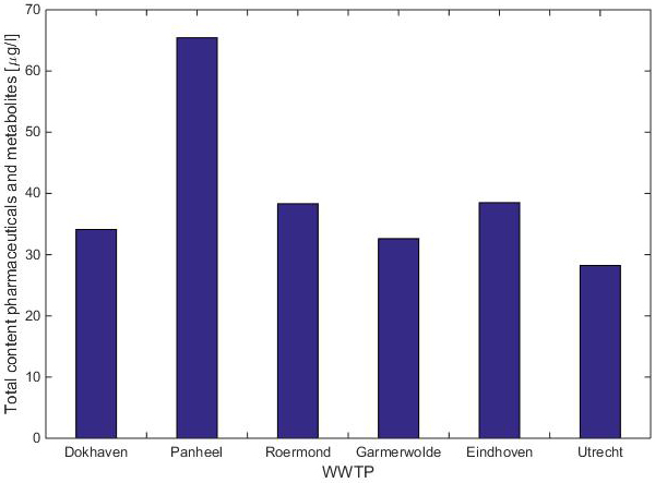
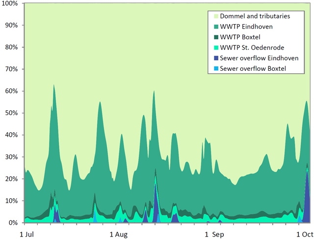
Figure 1. Total count of drugs and their metabolites in the effluent of the Panheel sewage treatment plant

Various techniques have been developed to purify drinking water in recent years, but it would actually be more effective to remove such substances at the source (think of households and hospitals). An end-of-pipe solution after the sewage treatment is also an option: good for the environment and also beneficial to the drinking water production.

In principle, techniques like advanced oxidation, which is used in drinking water production, could also be suitable for the removal or conversion of medicines in waste water.
The problem, however, is that the residual water (effluent) of sewage treatment plants contains a lot of Effluent Organic Material (EfOM). As the structure of this material corresponds somewhat with that of medicines, the EfOM disturbs in the decomposition process. It competes with the medicines for adsorption positions in adsorption processes, for example with activated carbon. As a result, the removal from effluent becomes relatively inefficient. In addition, harmful by-products could be created by reactions of the EfOM.

The project that is described in this article, examined whether it will be technically and possibly also economically more feasible if EfOM is removed (partly) via a separate pre-treatment. For this purpose, experiments were first performed on laboratory scale with two different pre-treatment methods and several advanced oxidation processes (AOPs) as the next step. On this basis, a pilot plant was built at a sewage treatment plant, where research takes place on a larger scale.

Effluent pre-treatment

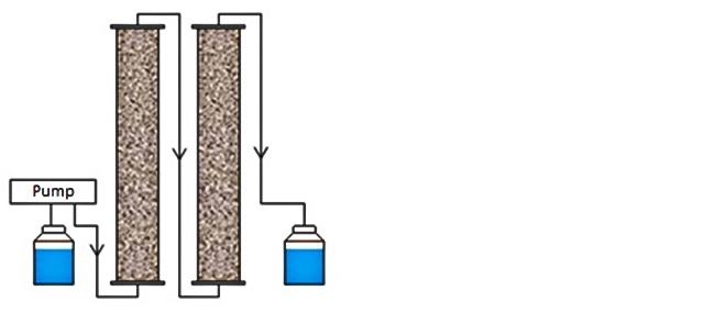
The research was carried out with the effluent of the Panheel sewage treatment plant, in which relatively high concentrations of medicines occur. Here, two different types of pre-treatments were applied:

• Ion Exchange (IEX): the water is filtered through a column with a resin that can filter negatively charged ions from the water.
• Ozone/bio-filtration (O₃/bio-filtration): treatment with ozone allows for partial oxidation of certain compounds, which can then be broken down further using micro organisms.
The EfOM consists of various organic material groups, and both pre-treatment techniques have a different influence on these groups (table 1).


Table 1

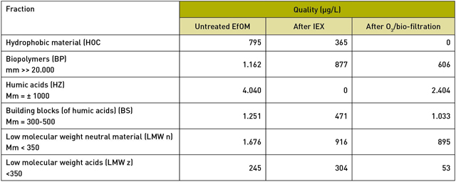
IEX appears to remove all the humic acids from the effluent. In addition, this treatment technique removes about half of the hydrophobic material, 60 perc ent of the building blocks and a quarter of the biopolymers.
O₃/biofiltration has a very different effect. This technique removes all hydrophobic material, about half of the biopolymers, 40 per cent of the humic acids and about 20 per cent of the building blocks. So, a big difference.

Advanced oxidation as next step

Advanced oxidation (AOP) uses highly reactive hydroxyl radicals, able to break down a wide range of organic compounds. For example, hydroxyl radicals are formed in a UV/H₂O₂ process. With this process medicines can be broken down in two different ways:
• Depending on the wavelength being used, some molecules can absorb UV radiation and then fall apart. This process is called photolysis.
• H₂O₂ can also absorb UV radiation and then break down into two hydroxyl radicals (• OH). These hydroxyl radicals can then oxidise many types of organic compounds.

UV radiation is often used to disinfect drinking water. An important parameter in UV processes is the amount of UV energy, also called the dose. Advanced oxidation requires about ten times as high a dose than that which is needed for disinfection. In addition, the water of a sewage treatment plant is badly permeable to UV radiation, rendering the UV process very ineffective.
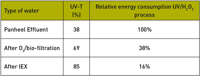
By removing (part of) the EfOM from the effluent, the water becomes more permeable to UV radiation, as a result of which the energy consumption of the UV process is greatly reduced (table 2).


Table 2

Initially, a mixture of more than 30 medicines and some control substances like caffeine were added to the Panheel effluent, and the effect of the different treatments on the effectiveness of a subsequent advanced oxidation process was studied on a laboratory scale. Not only the conversion of the added micro-pollutants was looked at, but also the degradation and formation of some (known) metabolites of drugs (which, incidentally, were not dosed).
The investigation indicated that after a pre-treatment using IEX at a dose of 300 milljoule (mJ) per square centimetre, most medicines were already degraded to concentrations below the cut-off. In comparison: an advanced oxidation process usually needs at least 500 millijoule per square centimetre.
This means the UV/H₂O₂ process is very efficient at applying a pre-treatment with, for example, IEX, not only because a low UV dose suffices, but also because relatively little energy is required to reach that dose (see table 2).

In addition to the above oxidation process based on UV/H₂O₂, experiments were also performed in the laboratory with other oxidation processes, such as O₃/H₂O₂ and O₃/UV.

On the basis of the results, it was decided to conduct a pilot experiment on the Panheel sewage treatment plant, in which both pre-treatment processes would be studied side by side, each followed by a UV/H₂O₂ process and an activated carbon filter. This filter is intended primarily to eliminate the excess H₂O₂, but also as an additional barrier, because, after all, a relatively high concentration of medicines was dosed in the research. Here, too, a similar improvement of the UV-T, and thus of the UV/H₂O₂ process, was found throughout the duration of the experiment (approximately three months).

Optimising the purification process

The experiments' results indicated that the removal of part of the EfOM did in fact lead to a much more efficient UV/H₂O₂ process on a larger scale, with a significantly lower energy consumption. This effect is the greatest with a pre-treatment with IEX, but that is countered by the fact that its application generates a concentrated waste stream with a high salt concentration, which may probably not just be discharged, and that may also still contain traces of drugs. Extra costs will have to be incurred for the processing of this concentrate. The pre-treatment with O₃/bio filtration doesn't have this disadvantage.

Furthermore, the investigation showed that metabolites can also be properly converted in the tested processes, and that a higher conversion is generally found after pre-treatment. At the same time, this shows that additional metabolites are formed in some cases during the oxidation process. In applying a lower dose, the original medicines are sufficiently converted, but other undesirable products, such as carbamazepine-10,11-epoxide, may be formed.

This is also a trade off that should be taken into account in a decision to implement such a process widely. What dose delivers an acceptable result at the lowest possible cost? This is a policy question for the District Water Boards. Because the current analysis techniques are so good, there is always something that can be shown, the question of which low levels are acceptable has more to do with politics and imaging than with risks for the environment and public health.

Of course, the expected cost plays a large role in any optimisation. A report by the Foundation for Applied Water Research (STOWA) indicates that ozonisation in combination with downstream sand filtration would cost approximately 0.2 to 0.3 Euro per cubic meter. Using the CoP cost Calculator by Royal HaskoningDHV, a first indicative estimate was made of the additional costs that the pilot set-up processes would incur. This estimate shows that the costs for these processes are about the same as the above mentioned processes. It still didn't take into account the increased efficiency of the UV/H₂O₂ process, generating a considerable saving on energy consumption and possible chemicals that may be necessary for this process.

Conclusions

• The effluent of sewage treatment plants still contains significant quantities of drugs and their metabolites.

• With advanced oxidation processes such as UV/H₂O₂, these organic micro pollutants can be broken down efficiently if the EfOM is (partly) removed first.
The two tested pre-treatment techniques are both suitable. Pre-treatment with ion exchange generated the greatest energy gains for the process, but it generates a salty waste stream (with a part of the drugs), which will have to be treated afterwards. Pre-treatment with O₃/bio filtration offers less energy savings, but also no concentrate, and also removes a part of the medicines. This technique, however, is slightly more sensitive to disturbances.

• Optimisation of the processes should also take the possible formation and conversion of degradation products/metabolites into account. In addition to technical optimisation, imaging and cost also play an important role.

• The additional costs for such a combination of the studied processes, appear to be of the same order as that listed in the STOWA report. Because pre-treatment significantly improves the water quality for an advanced oxidation process, extra cost savings may probably be possible here.

Roberta Hofman-Caris
(KWR Watercycle Research Institute)
Wolter Siegers
(KWR Watercycle Research Institute)
Kevin van de Merlen
(AWWS)
Ad de Man
(WBL)

Summary

Drugs ending up in a sewage treatment plant via the sewer water, are only partly broken off there. As a result, residue remains in the surface water. Techniques to purify drinking water are often less effective in wastewater because it contains a lot of organic material. By removing a large part of this first, it is possible to convert medicines much more effective by using advanced oxidation processes. Although two purification processes are then required, this can be a cost saving compared to previous estimates, making treatment of waste water not only technically, but also economically more feasible. This was the result of a study at the Panheel sewage treatment plant in Limburg.

Literature

Mulder, M., Antakyali, D., Ante, S. (2015). Verwijdering van microverontreinigingen uit effluenten van RWZI’s; Een vertaling van kennis en ervaring uit Duitsland en Zwitserland. STOWA-rapport 2015-27.

Hofman, J., Laak, T.t., Tolkamp, H., Diepenbeek, P.v. (2013). Geneesmiddelen in de waterketen in Limburg: herkomst en effect. H₂O-online 09-12-2013

Hofman, J., Tolkamp, H., Laak, T.t., Huiting, H., Hofman-Caris, R., Diepenbeek, P.v. (2013). Terugdringen van geneesmiddelen in de waterketen van Limburg. H₂O-online 10-12-2013

^ Back to start

Monitoring fish communities using DNA
on large rivers

Water managers need to monitor their fish communities. Until recently, use was made of data from commercial fishing. Since this is now subject to restrictions, an alternative is required. Not by catching the fish, but by showing the presence of their DNA in the water: environmental DNA.

The European Water Framework Directive (WFD) requires water boards and Rijkswaterstaat (part of the Dutch Ministry of Infrastructure and the Environment) to investigate their fish species composition and abundance. Until recently, Rijkswaterstaat made use of (fish trap) catch data of the commercial eels fisheries, the so called passive fish monitoring programme, to map the species composition in public waters. Due to the largely disappearing commercial eel fishing on public waters, the passive fish-monitoring programme is under pressure. An alternative investigation method for the WFD is therefore required.

eDNA

A possible alternative which is now investigated by the Rijkswaterstaat is the eDNA method (eDNA = environmental DNA). This method is based on the fact that all (aquatic) organisms excrete DNA in their environment. This can be in the form of faeces, mucus, urine, scales etc. By taking water samples, this DNA, which is freely present in the environment, can be 'caught' and the present species-specific DNA can then be indicated. On the basis of this analysis it is possible to determine from which organism the DNA is originating
The eDNA-method indicates the presence of fish species. The method is (still) inconclusive as to numbers (by length class) or biomass.

The eDNA technique is still in development. One of the uncertainties is that it is not yet exactly known what sampling protocol ensures reliable results. Another point is that the eDNA as found in flowing waters may originate from elsewhere. After all, eDNA remains intact for several days to weeks.
This research is a first exploration into the applicability of the eDNA method in large Dutch rivers. A comparative field study was implemented for this purpose, in which the results of the regular fishing traps were compared to those of the eDNA method.

Set-up of a comparative field study

The traditional fish trap fishing was compared to the eDNA method on a trajectory in the Gelderse IJssel near Deventer. Fishing was done using fish traps and water samples were taken at this location on three consecutive days. The water samples were analysed for the presence of DNA of six fish species: two common (perch and roach), two less common (ide and bleak) and two more rare (catfish and river bull-head).

In this research three sets of fish traps were used distributed over approximately 4.5 km. Water samples were taken at four locations on the same trajectory: directly upstream from each trap and on 1.5 kilometres downstream of the trap furthest downstream. To also map the distribution of DNA samples over shorter distances, a total of nine water samples were taken at each location (of 2 litres each), spread over three transects, 150 metres away from each other. Three water samples were taken per transect, at places with a different depth (one, two and five metres).

The analyses were carried out with the qPCR method by which it is possible to detect the presence and quantity of (e)DNA. The required tools – the primers and probes – were successfully developed and validated in this study.

Results

Of the six target species, four were found in the fish traps during the study period (table 1). This is, moreover, due to the large number of fish traps that were used. With only one trap, we caught a maximum of three target species in three days. If all three locations were sampled, but on only one day, we would likewise have ended up with a maximum of three target species.


Table 1

All six target species were observed with the eDNA method. The observed eDNA concentrations differ greatly between the species (Figure 1). The distribution of the common roach has the largest spread, that of bleak the least.


Figure 1. Boxplots of qPCR values of all measuring points on all days per species. Note the difference in scale on the y-axis


Figure 2. eDNA distribution map of perch. Per day for each measuring point the average qPCR value is shown. The larger the circle , the more eDNA is found in the water sample. For each measurement location nine measuring points on three transects are clustered. The measurement locations are approximately 1.5 kilometers apart. The arrow indicates the direction of flow


Figure 3. eDNA distribution map of Wels catfish. Per day for each measuring point the average qPCR value is shown. The larger the circle , the more eDNA is found in the water sample. For each measurement location nine measuring points on three transects are clustered. The measurement locations are approximately 1.5 kilometers apart. The arrow indicates the direction of flow

If eDNA is found in a water sample, it is assumed that the species is present at the measuring point. This is how eDNA distribution maps are created. The eDNA-distribution maps for perch and catfish is given as an example in Figure 2 and 3.

Perch was observed in 97 of 108 water samples (90 percent) with qPCR values up to 4988 DNA copies per litre. The distribution of catfish eDNA shows a different pattern. Catfish was only observed in 31 of 108 water samples (29 percent) with qPCR values up to 834 DNA copies per litre. Catfish wasn't found in the trap catches.

The distribution maps show that perch and catfish were observed every day at each cluster of nine measuring points – a single sampling location. All species that were found in the traps were also shown with eDNA. Catfish and river bull-head were not found in the fish traps, but were shown with the eDNA method.

This study shows that it is possible to show the presence of common and less common species, such as catfish and river Bull-Head, with the eDNA method. Compared to fish trap fishing, the eDNA method provides a greater chance of observing a species.

By taking water samples at multiple locations this research resulted in maps of the distribution of eDNA (in space and time). In this way better insight is gained in the probability a target species is observed by the eDNA method. The distribution maps also give information on the origin of the eDNA.

False negative observations

The distribution of eDNA differs per species. eDNA of catfish was found at far less measuring points than perch. If eDNA appears to be less distributed in water, the observation chance (the chance of finding the eDNA of a species) also diminishes. Not finding a species with eDNA while the species is present, is called a false negative observation. For catfish, the chance of a false negative observation is greater than for perch.
Insight into the species-dependent distribution of eDNA in flowing waters is required to handle a sampling strategy that minimises the chance of false negative perceptions.
On the eDNA-distribution maps (such as Figure 3 and 4) one can see that regardless of the day, a random measurement location could have been sampled to observe all six target species. The chance of false negative observations would have been greater with less water samples per measurement location, because eDNA wasn't found of most of the target species at all measuring points.
On the basis of these results, it was concluded that the observation chance is high enough for the eDNA method to be considered a suitable alternative to passive fish monitoring.

False positive observations

At the same time, with rising eDNA observation chances, the chance that the picked up eDNA originates from outside (upstream) the research trajectory, may increase. Because, earlier research showed that eDNA can be detected kilometres from the (fish) source. The probability of so called false positive observations affects the interpretation of the results and thus the applicability of the eDNA method. This applies, for example, to research in the context of the European Water Framework Directive and to the distribution of exotics.
The eDNA distribution maps also offer a solution here. The source of eDNA can be determined by comparing the amount of eDNA with each other on two consecutive measuring points (or strips). For catfish, we see less eDNA upstream from different measuring points than on the measuring point itself, which indicates a DNA source between these two measurement points and thus the presence of catfish.

Conclusions

The main conclusions from this research are:
• The presence of common and less common fish species on large rivers can be indicated with the eDNA method;
• The eDNA method offers a greater chance of observing a species than fish trap fishing;
• eDNA distribution maps offer insight into the likelihood of observing a species and in the origin of eDNA;
• The eDNA method is practically feasible and less labour-intensive than the fishing traps, yet assures reliable results;
• The eDNA method seems to be a suitable alternative to the passive monitoring programme.

To be suitable as an alternative to passive monitoring requires a reliable, efficient and secure method for all fish species. Although common and less common species were included in this study, it is necessary to understand the observation likelihood for the entire fish community. To this end, the eDNA-meta bar coding technique can also be a good addition. Using this non-quantitative DNA method, a picture of the total fish community can be achieved. However, more knowledge of the behaviour of eDNA in water is required so as to reduce the chance of false positive observations.
These two research questions can be answered with basic research and/or the use of computer models. However, this is very time consuming and labour intensive. In addition, the quantity and distribution of eDNA in water can be determined by many factors, which may vary greatly in space and time. Therefore, a more pragmatic approach is preferred with this exploratory study as a starter. By choosing the combination of qPCR and the measuring points well, it is possible to make the distribution and origin of eDNA (under the prevailing environmental factors) more transparent. This increases the reliability of the results, and fundamental research into the behaviour of eDNA in flowing waters is less required.

Wouter Patberg
(Koeman en Bijkerk )
Jan Warmink
(Sylphium molecular ecology)
Hans Ruiter
(Public works and water management)
Bart Wullings
(KWR Watercycle Research Institute)
Edwin Kardinaal
(KWR Watercycle Research Institute)

Summary

The European Water Framework Directive (WFD) requires water boards and Rijkswaterstaat to investigate the fish communities. Due to the largely disappeared commercial eel fishing in public water, passive fish monitoring (using data of the fishermen) came under pressure.

The eDNA method (eDNA = environmental DNA) could be an alternative. This method is based on the fact that all (aquatic) organisms excrete DNA. By taking water samples, this DNA present freely in the environment, can be 'caught' and on the basis of analysis, it is possible to determine from which organism the DNA originated. The research that is described in this article shows that the eDNA method can be suitable as alternative to catching and counting the fish itself.

^ Back to start

Polder water quality

A knowledge jump
from high-frequency monitoring

The water level in the Netherlands is mainly regulated by pumping stations. Pumping stations are traditionally also the location to monitor water quality. During the last decades, more and more pumping stations have been equipped with automatic switching systems and run predominantly during the night hours, while the water quality is still mostly measured during the day. According to research, this can have a substantial impact on reported trends in water quality.

The De Blocq van Kuffeler pumping station is one of the four pumping stations that keep the Flevo polder dry. Deltares established a monitoring station in September 2014 in collaboration with the Regional Water Authority Zuiderzeeland, which measures the concentration of nitrate (NO3), total phosphorus (TP) and suspended sediments (SS) in the Lage Vaart, every five to ten minutes. It is the world's first high-frequency monitoring station for water quality at a pumping station. The drainage area of the Lage Vaart is used mainly for agriculture.

The dynamics of nitrate

The nitrate concentration at pumping stations seems to be related to drainage water from the agricultural area in the polder. The measurements indicated a low nitrate concentration at the pumping station during the period from 1 October to mid-November and from about mid-April to the end of August. During these periods, the groundwater levels were lower than the tube drainage level. During intense rainfall events in the summer and prolonged wet periods in the winter, the groundwater level increases to up to or above the tube drainage level, and an increase in nitrate concentrations is measured at the pumping station about five days after a rainfall peak.
It was already known that the nitrate concentration in the drainage water in the Flevopolder is relatively high (with concentrations measured between approximately 5 and 20 milligrams N per litre). As a result of the shrinkage cracks in the Flevopolder's clay soil, there is a rapid discharge of nitrate when the groundwater levels reach the level of the drainage tubes.
Our measurements indicate that this drainage water controls the quality of surface water to a large extent under wet conditions.

Effects of manure spreading

In order to get better understand the sources and transport routes of nitrate, a survey was conducted to examine whether a relationship can be established between the high-frequency concentration series of nitrate and the precipitation (hourly data), using time series analysis (a transfer function-noise model). These results are shown in figure 1. The top graph shows the measurements and the modelled concentration time-series, the lower figure shows the residuals (measurement minus model). The time-series model indicates that 70 per cent of the dynamics in the nitrate concentration can be explained by a reaction to precipitation. The results indicated that the decline in the concentrations during dry periods were properly modelled. The wet periods show varying results: the increase in concentration was properly modelled in December; in January, the concentration was overestimated, while the concentration was underestimated in February/March.


Figure 1. High frequency measuring set for nitrate, precipitation (sum of the previous 24 hours) and the time-series analysis model

Differences between the modelled and measured concentration give additional insight into the nitrate dynamics in the Flevopolder. The overestimation in January is probably the result of dilution due to heavy rains in combination with a decrease of in the NO3 stock stored in the soil profile due to leaching with rain during previous month. This effect is not included in the transfer model. The underestimation and especially the peaks in measured concentration in February/March can be explained by manure application in that period.
The Manure Law allows for spreading of manure on arable land from 1 February and 15 February on grassland. The first three weeks of February 2015 were dry. It is likely that manure was applied to land on a large scale during this period. On 20 February, it started raining heavily and a few days later, on 24 February, the nitrate concentration peaked at almost 10.5 milligrams N per litre. The measured nitrate concentration was also higher than the modelled nitrate concentration during the subsequent rain showers in late February and early March.

Total-phosphorus dynamics

While it is quite simple to a indicate a dominant source for nitrate, the same can not be said for total phosphorus (TP). The concentration at the pumping station increases structurally during dry periods and is at its highest in the summer. This indicates the influence of phosphate rich groundwater and a later release of phosphate from the water bottom. Other sources of phosphorus are phosphate rich water from the Oostvaardersplassen and the sewage treatment plant at Almere, who discharge on the Lage Vaart.
The nitrate rich agricultural water, which has a huge impact on the water quality during wet conditions, contains notable low TP concentrations (Figure 2). The precipitation on 10-12 December led to a peak in the nitrate concentration of 5.5 milligrams N per litre on 17 December.


Figure 2. Dynamics in nitrate, total-phosphorus concentration and suspended solids (as turbidity) after a wet period on 10, 11 and 12 December, with the precipitation and the pump regime

Aside from the peak in TP concentration during the initial stage of pumping, the concentration on 17 December was less than on 11 and 12 December. Although it cannot be excluded that the drainage water from rural areas contains increased phosphorus concentrations, this cannot be seen at the pumping station. There may be leaching of phosphorus from agricultural soils to surface water during wet conditions, but it will not be transported directly to the pumping station.
A part of the phosphate in the soil that will be leached to the surface water is bound to fine particles. In addition, dissolved phosphate will be attached to iron oxide particles in surface water that are formed in the ditch by seepage of ferrous groundwater.
Sedimentation of these forms of particular phosphorus in the ditches and channels prevents rapid transport to the pumping station. Sedimented phosphorus can lead to a later release of phosphate from the bed sediments to the surface water in the summer, thus creating a 'delayed' release. The high ortho-P concentrations during the summer indicate a late release of P from the bed sediment.
Such conversion processes and the temporary storage of phosphate doesn't make it any easier to quickly determine the effects of agriculture practice and manure measures on phosphorus concentration in the surface water.

The effects of pumping

Previous research in Friesland has already indicated that nutrient concentrations could increase during pumping. We were able to better quantify this effect using the high frequency TP and SS measurements at the De Blocq van Kuffeler pumping station. The TP and SS concentrations increase suddenly when the pumping station is in operation (see Figure 3 for TP). The TP concentration increases 0.06 mg P per litre on average over a year when pumping with one pump; this becomes 0.13 mg P per litre when pumping with two pumps. The concentration of suspended sediments increased on average by 4.4 milligrams per litre when pumping with one pump, while this was 22 milligrams per litre when pumping with two pumps.


Figure 3. Change of the TP concentration during pumping

This increase when pumping indicates that the change in flow rate of the water leads to resuspension of sediment-bound P from the water bottom.

The increase in TP concentration during pumping was much smaller in the surveyed polder than what was measured during wet periods in 'free-drainage' areas in the Netherlands or beyond, where concentration increases were reported with a factor of 100 or more. Because the flow rate of the water in polders is limited to the pumping capacity of the pumping station, the risk of resuspension of large amounts of P is also limited. Polders therefore have a large capacity for storing P in the surface water system. As a result, the risk of releasing P from the water bottom at a later stage, and thus for higher concentrations in summer, is much greater for polders than for free-drainage areas.
The De Blocq van Kuffeler pumping station runs mostly in the evening and at night because power is then cheaper. Water quality samples are always taken during the day. This leads to an underestimation of the TP concentration of the water that was actually pumped water. This has implications when determining the loads from the 'Lage Afdeling' to the Markermeer and possibly also for trends in water quality.
In 2008, the pumping station was converted from a manually operated, diesel engine powered pumping station, to a fully automatic, electric motor powered pumping station. It looks pretty much like this transition can be seen in the TP concentration time series (Figure 4). The time series from 2000 to 2015 indicate a declining concentration. The time series from 2000 to 2009 and from 2009 to 2015, however, indicate increasing concentrations. These differences are caused by the sudden reduction in TP concentration at the beginning of 2009, exactly the time that the pumping station was converted. Although it may not be entirely excluded that there are other causes for the sudden decrease in TP concentration, it is likely that this has to do with the change to pumping during the evening and at night.


Figure 4. TP concentrations time series, the LOWESS trend and slope

In the past twenty years, a large number of pumping stations in the Netherlands were converted from diesel powered to fully automatic electric pumping stations, mainly operating during the evening and night hours while sampling takes place during the day. It is therefore conceivable that the change in pump regime on a regional and even national scale, may have an effect on reported trends in water quality of the actually pumped water. Sampling of water quality with grab samples during the daytime at pumping stations that run primarily at night, lead may to an underestimation of export loads of substances that have a high affinity for binding to sediments.

A comprehensive article on the described research will shortly appear in the magazine Hydrology and Earth System Sciences.

Bas van der Grift
(Deltares)
Joachim Rozemeijer
(Deltares)
Hans Peter Broers
(TNO Geological Survey of the Netherlands)
Wilbert Berendrecht
(Berendrecht Consultancy)
Michiel Oudendijk
Zuiderzeeland Water Board

Summary

Water levels are regulated with pumping stations in around 60 percent of the Netherlands. They pump excess water onto the polders. The water quality is often measured at these pumping stations. Sampling of water quality during the daytime with grab samples at pumping stations that run primarily at night, leads to an underestimation of the pumped quantities of substances, like phosphate and suspended sediments.

Concentrations can now be measured at high frequency using new measurement techniques, allowing one to get a much better picture of the origin of certain substances and the nature of the transport processes. High frequency measurements at the De Blocq van Kuffeler water pumping station in the Flevopolder have indicated that nitrate from agricultural areas is drained away relatively quickly in wet periods, but that phosphate is actually retained much more in polder systems than in free drainage areas. Phosphate emissions occur, therefore, not predominantly in winter, but due to the later release from the bed sediments and by feeding from the ground water, rather in summer.

^ Back to start

Swimming in a canal:
is the risk predictable?

Even Queen Máxima does it. Jumping into the canal in a wetsuit, swimming for charity. However, a city canal is no bathing location. Can a water board nevertheless estimate the expected water quality and recommend whether or not to allow such an event to proceed? De Dommel water board developed its own model and dared to advise in 2015.

City canals are increasingly hosting big swimming events. Such swimming events also take place in the city canals of 's-Hertogenbosch, managed by water boards De Dommel and Aa & Maas: the Swim to Fight Cancer (STFC).
However, a dilemma remains. A canal is not a bathing site, but the water board cannot prevent people from jumping in. At the same time, the water board also happens to be the water quality administrator and therefore feels responsible for the hundreds of swimmers.
What to do? Given the social relevance, De Dommel water board finally decided to cooperate behind the scenes in providing insight into the quality of the water at the time of the event.

What is known about the water quality in the canals of 's-Hertogenbosch? Not much because the swimming route isn't bathing water. What is known is that different wastewater treatment plants and sewage overflows discharge upstream in the Dommel. In order to better understand the water quality, a measuring programme was established, measuring at two locations. The last sampling is two days before the go-no go-decision and four days before the start of the event. However, in this period, the water quality can change significantly due to rainfall events and discharges.

Model

Therefore there is a need for a tool to bridge this period of four days to be able to improve advise on water quality. This was the reason for developing a water quality model with the purpose of simulating the water quality as accurately as possible during the event.
During the model development, the central questions were :
- Which bacteria sources upstream have the largest influence on the water quality of the swimming trajectory?
- What are the travel times of the most important sources up to the swimming trajectory?
- What are the expected concentrations of bacteria in the swimming trajectory on the day of the swimming event?

It was decided to develop the water quality model in Sobek-1DWAQ to answer these questions. The water board already uses Sobek-1D/2D for hydrological calculations.

The water system

The Dommel river originates in Belgium and enters the Netherlands south of Eindhoven. The water flows towards 's-Hertogenbosch through Eindhoven, Sint-Oedenrode, Boxtel and Vught, among others. This is where the Dommel merges with the Aa and they form the Dieze, which eventually flows into the Maas.
The two kilometre long swimming trajectory of the Swim to Fight Cancer starts in the Singelgracht and then goes through the Dommel to the finish in the Dieze. Upstream from the swimming trajectory, three sewage treatment plants discharge treated waste water into the Dommel. There is also a good number of overflows in place, discharging a lot of untreated waste water during heavy rain. The water quality of the swimming trajectory is therefore largely determined by the water quality of the Dommel.

Structure of the model

The water board has developed a model to identify the main sources and to make bacteriological calculations. This model was calculated for the summer period of 2014.
In step 1, a hydrodynamic model was established that included the trajectory of the Dommel from Eindhoven to' s-Hertogenbosch. The modelled water system consisting of the A water courses (streams and tributaries) and the different structures. The various sources were filled on the basis of measurement sets for 40 municipal sewage overflows, the three sewage treatment plants and the drainage from the rural area.
The water quality model was developed in step 2. Different sources were labelled to do a tracer calculation. In addition, the sources were given a concentration of the bacterium Escherichia coli (E. coli), found in human and animal faeces, based on available measurements and literature values. For the overflows and sewage treatment plants, this is 100,000 colony forming units (CFU) per 100 ml, for the rural drainage: 100 CFU per 100ml. The default values in Sobek-WAQ were used for the calculations of the decay rate of the bacteria.

Source analysis

In periods of dry weather, about 20 percent of the water in the swimming trajectory consists of effluent of the three sewage treatment plants, the other 80 percent is water of the Dommel upstream from Eindhoven and the tributaries of the Dommel. With summer showers, the share of water from sewage overflows and sewage treatment plants increase, these are the peaks in Figure 1. With rainfall, the share of water from sewage overflows varies between 2 and 20 percent. Then 40 to 60 percent is effluent water from sewage treatment plants and the remaining 40 to 60 percent is water from the Dommel upstream from Eindhoven and tributaries of the Dommel.


Figure 1. The contribution of the sources of water on the swimming trajectory

The source analysis has indicated that the Eindhoven sewage treatment plant and the overflows from Eindhoven and Boxtel represent the largest part of the water in the swimming trajectory. Furthermore, it appears that numerous overflows have occurred in this period of three months. The conclusion is that a few sources will determine the water quality on the swimming trajectory. The travel time from the source to the swimming trajectory was established for these sources in the next step.

Travel times

An overflow event at Eindhoven generates a narrow and high drainage peak in the Dommel and – over time – a wider and lower drainage wave on the swimming trajectory. This is evident from Figure 2. The time difference between the two drainage waves is the travel time of the water from the source to the swimming trajectory. The amount of rainfall, the current speed and the vegetation of the Dommel determine the spread in travel time.


Figure 2. Drainage waves of the Eindhoven overflows and the model calculation for the trajectory of the Swim to Fight Cancer 2015 in relation to precipitation (KNMI station Eindhoven)

The travel time for the sewage treatment plant and the overflows of Eindhoven ranges from 2 days to over 4.5 days (see the table). The travel time to the swimming trajectory varies from 1 to 2.5 day for the nearer sewage treatment plant and the overflows of Boxtel.
If it should rain within 4.5 up to 1 day prior to the start, leading to a discharge, then this has a negative effect on the water quality at the swimming trajectory.

Bacteriological calculations

Two measuring points were established in order to understand the water quality along the swimming trajectory, one at the start and one half way through the swimming trajectory. In total, fourteen times the E. coli concentration was measured in 2014, in the period from 1 July to 30 September. The swimming water standard (1800 CFU per 100 ml) was exceeded four times during this period (Figure 3).


Figure 3. Model calculation and water quality measurements on the swimming trajectory

The model calculations and water quality measurements corresponded very well, in general, especially for the run of peaks and in periods of dry weather. With overflow events, the model is still generating an underestimation of the E. coli concentrations, as on 10 August and 2 September 2014. However, both the model and the water quality research demonstrate that standards are exceeded in the swimming trajectory and that the Singelgracht in s-Hertogenbosch is therefore not always suitable for swimming. Furthermore, it appears that E. coli can be missed when sampling peak concentrations. The model provides insight on the E. coli concentration at any given time, making it a valuable addition to the water quality testing.

Value of the model

System knowledge was acquired with the model and the sources were analysed. The contribution of the sources along the swimming trajectory was shown. It was established that the Eindhoven sewage treatment plant, as the third largest sewage treatment in the Netherlands, had a huge influence. The Boxtel overflows are also relevant, especially due to the short distance to the swimming trajectory.
By determining the travel times, it is now possible to gauge shortly before the start of the swimming event if rain could lead to a deterioration in water quality.
A complete predictive model with a precipitation drainage model and data on paved surfaces for overflows, didn't appear to be feasible within the available time frame. It is necessary to continue to develop such a predictive model for the future.

Advice

On the basis of these findings, what advice could now be given to the Organisation of Swim to Fight Cancer?
The amount of rainfall in the week before an event is crucial for the water quality during the swimming. The water board will issue the forecast on water quality at the time of the event, two days before the starting shot. The basis for this advice is the water quality test, the weather forecast and the model analyses. After all, a lot of rain in the two days before the sampling probably means a bad water quality (Figure 4). If the weather remains dry from then, the water quality during the event will be just fine.


Figure 4. Time line important moments for the swimming event

Four days before Swim to Fight Cancer 2015, the E. coli concentrations were well below the swimming water standard. It was expected that it would rain a lot in Boxtel the day before and that possible overflows would take place. However, based on the model it could be concluded that these discharges would only pass through the route after the event. The water quality would therefore not pose a problem for the event. With that came the relieving words: it will go through!
The samples taken on the day of the event, confirmed the accuracy of this forecast afterwards. Many enthusiastic swimmers have swum the two kilometres and collected nearly 530,000 Euro for charity.

Henk Tamerus
(De Dommel Water Board)
Esther Vermue
(De Dommel Water Board)
Jan van de Graaf
(De Dommel Water Board)
Maaike Cazemier
(De Dommel Water Board)
Inge Folmer
(Royal HaskoningDHV)

Summary

Water boards do not want to promote swimming in non-official bathing locations. However, if hundreds of swimmers get into the water for charity's sake, the water administrator is still faced with a dilemma. The organisation of Swim to Fight Cancer 2015 asked De Dommel water board and Aa and Maas water board for advice. They gave advice behind the scenes by making the risks to swimmers clear.

Water quality testing alone is not sufficient in this case. Due to the analysis time of the samples, there is a gap of four days between sampling and the starting shot.

To bridge this gap, De Dommel water board has set up a water quality model. The model is an important tool for advising the organisation of the swimming event, because it removes the uncertainty in the last four days before the starting shot.

^ Back to start